Graphical User Interface (GUI)
To launch the GUI, run uq_physicell.
Note
This section of the GUI documentation is under active development. Content and usage instructions may change.
Example Workflow
This example demonstrates how to use the UQ PhysiCell GUI to perform a complete uncertainty quantification workflow: from model configuration to sensitivity analysis. We’ll build a simple model, run parameter sampling, and analyze the results.
Prerequisites: Navigate to your PhysiCell folder, populate the template project by running make template && make, then open PhysiCell Studio to customize the initial conditions and cell cycle model.
Step 1: Modify the Template Project Using PhysiCell Studio
Steps:
Enable the initial condition checkbox
Set the number of cells to initialize the model to \(0\)
Create and save the custom initial condition with a disc where \(R1 = 0\) and \(R2 = 200\)
Change the combo box from ‘Flow cytometry model (separated)’ to ‘live’ model
Add a mechanofeedback on cell cycle entry.
pressure decreases cycle entry from 0 towards 0 with a Hill response, with half-max 0.5 and Hill power 4.Save the .xml file
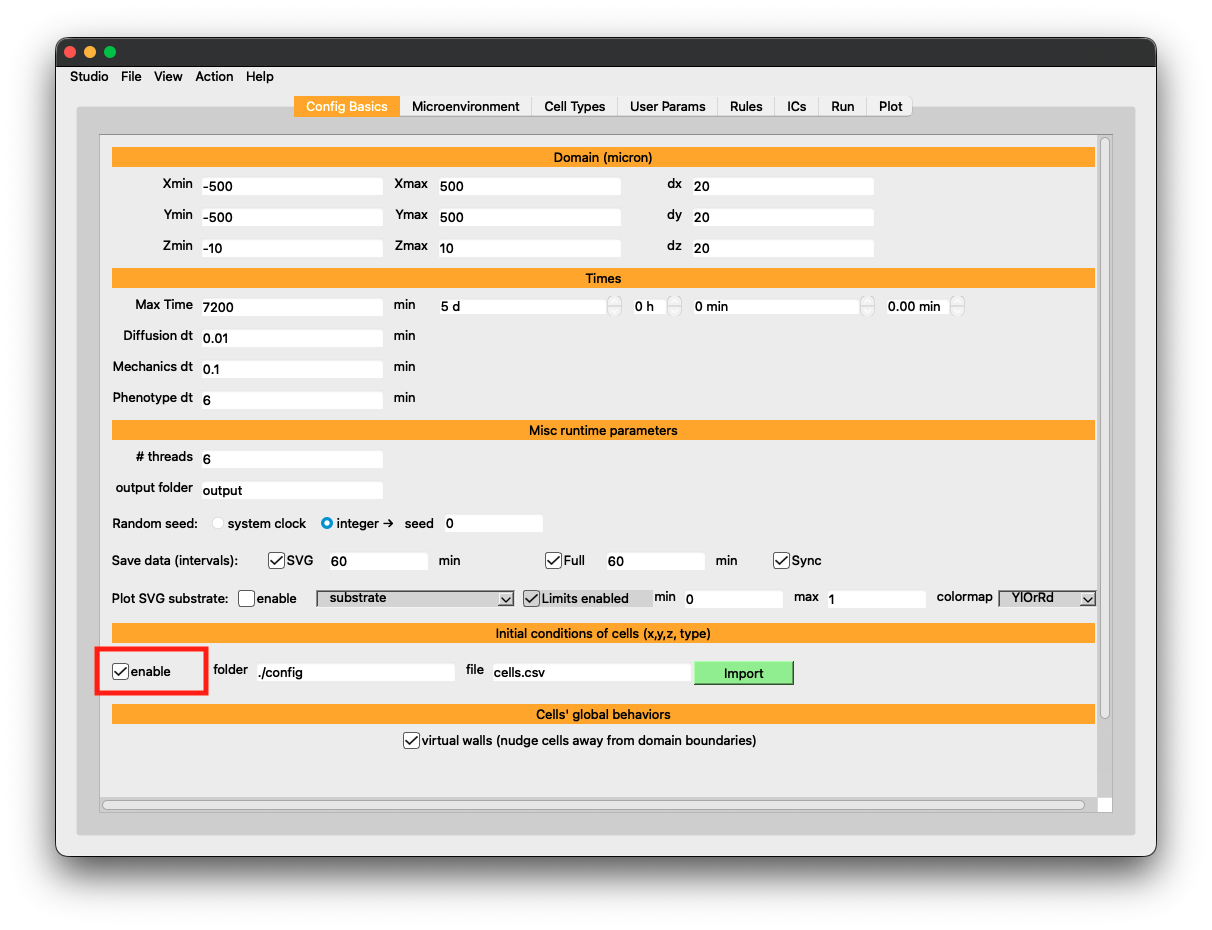
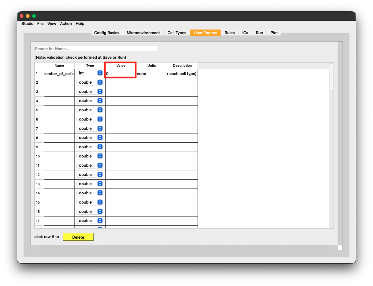
Left: Enable the initial condition checkbox (step 1). Right: Set the number of initial cells to 0 (step 2).
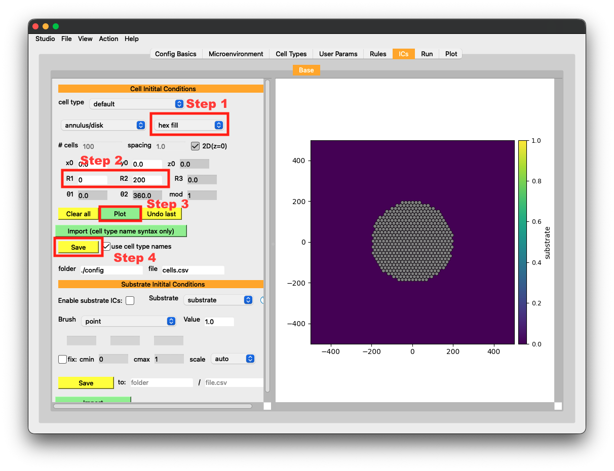
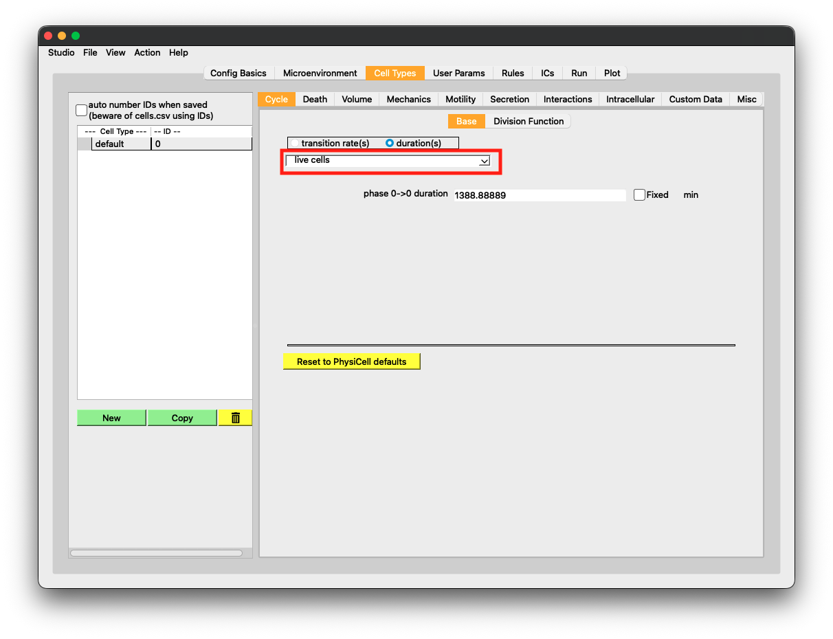
Left: Create a disc with $R1 = 0$ and $R2 = 200$, then save (step 3). Right: Change the cell cycle model to 'live' (step 4).
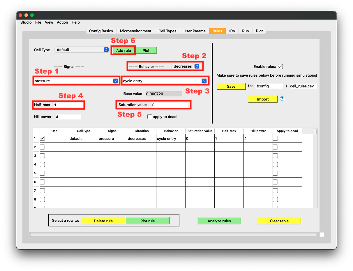
Create a rule `pressure decreases cycle entry from 0 towards 0 with a Hill response, with half-max 0.5 and Hill power 4` (step 5).
Step 2: Create the UQ PhysiCell Configuration File (.ini)
Now we’ll use the GUI to create a configuration file that defines which parameters to explore in our uncertainty quantification analysis.
Steps:
Launch UQ PhysiCell: run
uq_physicellin the terminalLoad the .xml file from your model
Select parameters to be fixed in the model exploration:
omp_threads= 1,enable SVG= false, andinterval= 240Select parameters to add to the analysis:
cell_cycle_entryandapoptosis_rateProvide a structure name (
Model A), executable path (project), and number of replicates (5)Save the .ini file (
uq_config.ini)
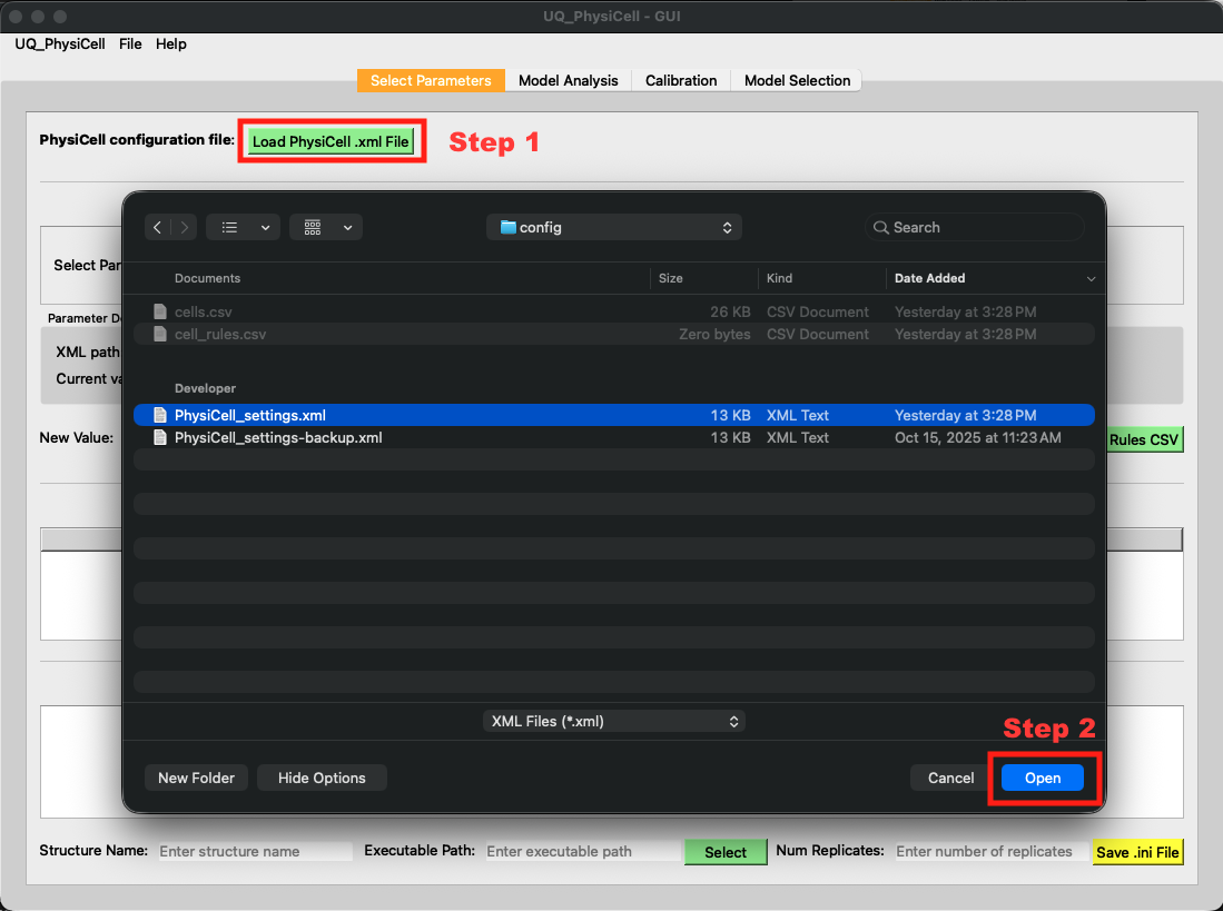
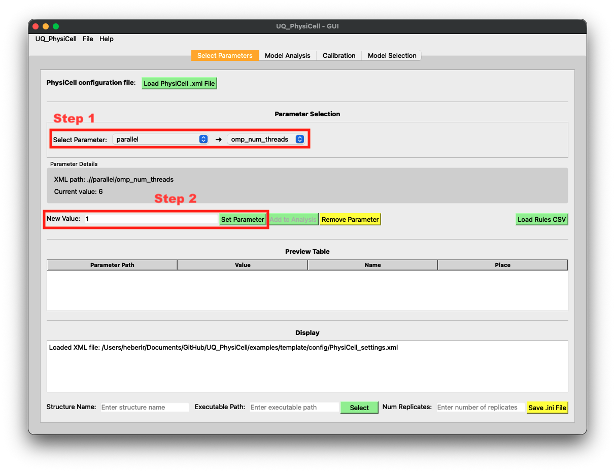
Left: Load the .xml file (step 2). Right: Set `omp_threads` = 1 (step 3).
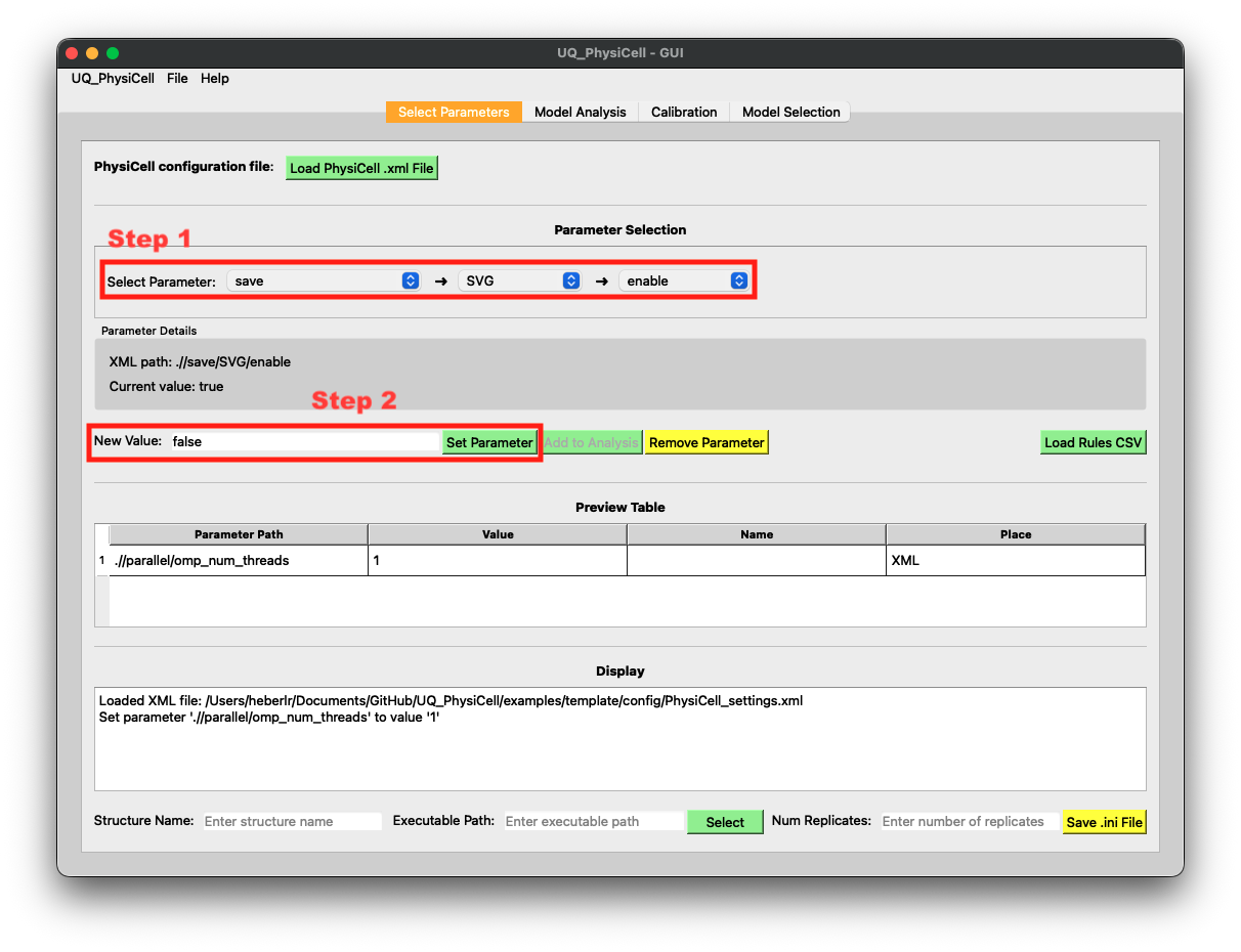
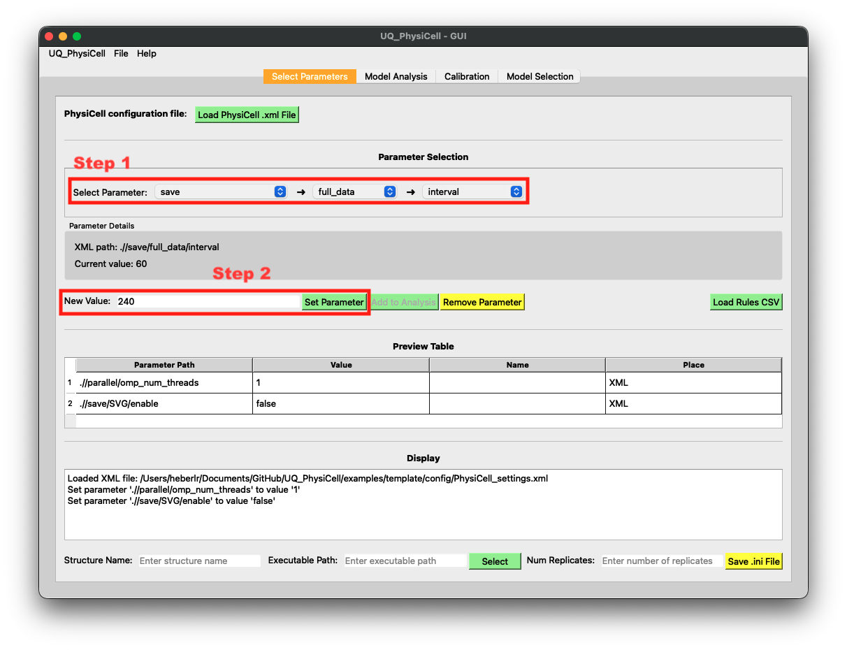
Left: Set `enable SVG` = false (step 3). Right: Set `interval` = 240 (step 3).
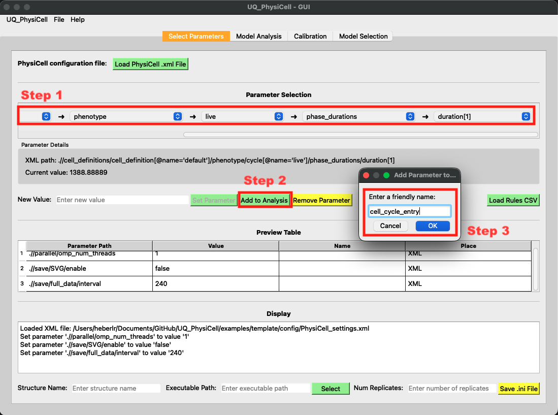
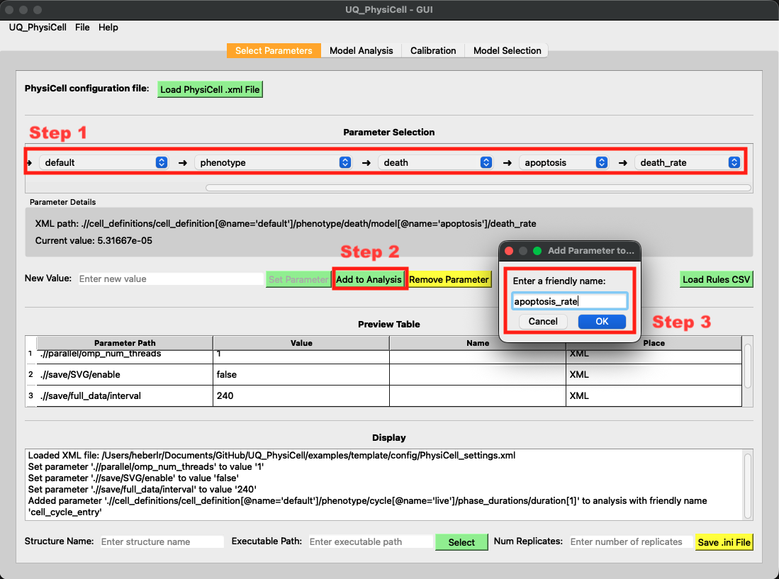
Left: Add the `cell_cycle_entry` parameter to the analysis (step 4). Right: Add the `apoptosis_rate` parameter to the analysis (step 4).
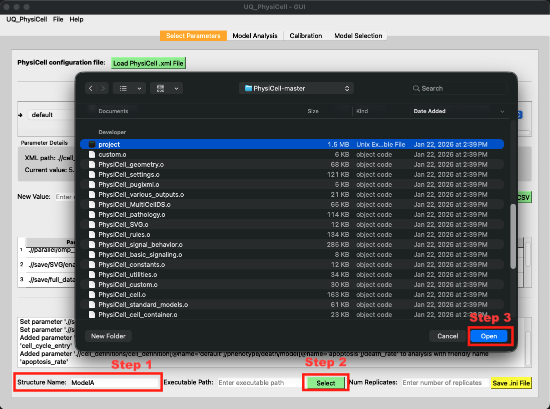
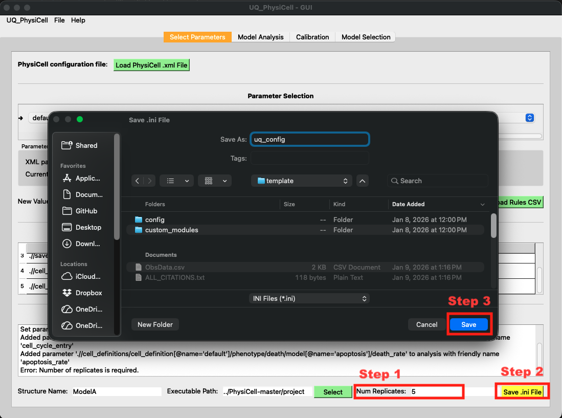
Left: Define the structure name as `ModelA` and set the executable path to `project` (step 5). Right: Set the number of replicates and save the configuration as `uq_config.ini` (step 6).
Step 3: Generate the Simulation Database (.db)
Next, we’ll sample the parameter space and run simulations to build a database of results.
Steps:
Define the parameter sampling strategy as
Globaland set the sampler toSobolCheck the range of the
apoptosis_rateparameter.Sample the parameters with
8samples and click Plot to visualize the parameter spaceSet the database filename to
Simulations.dband click the Run Simulations buttonSet the number of workers to run simulations in parallel using the inter-process strategy, then confirm in the warning message that you want to store the list of MCDS objects
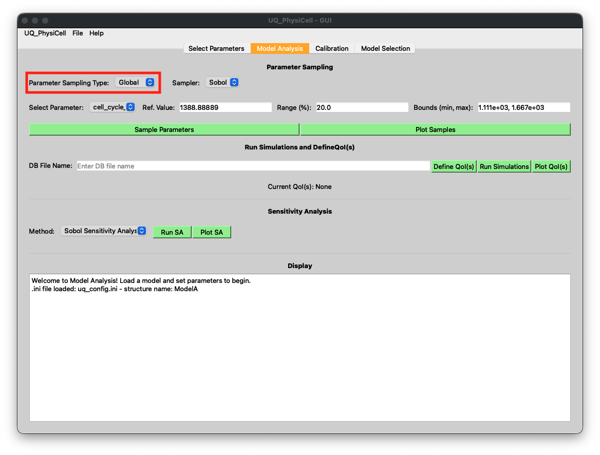
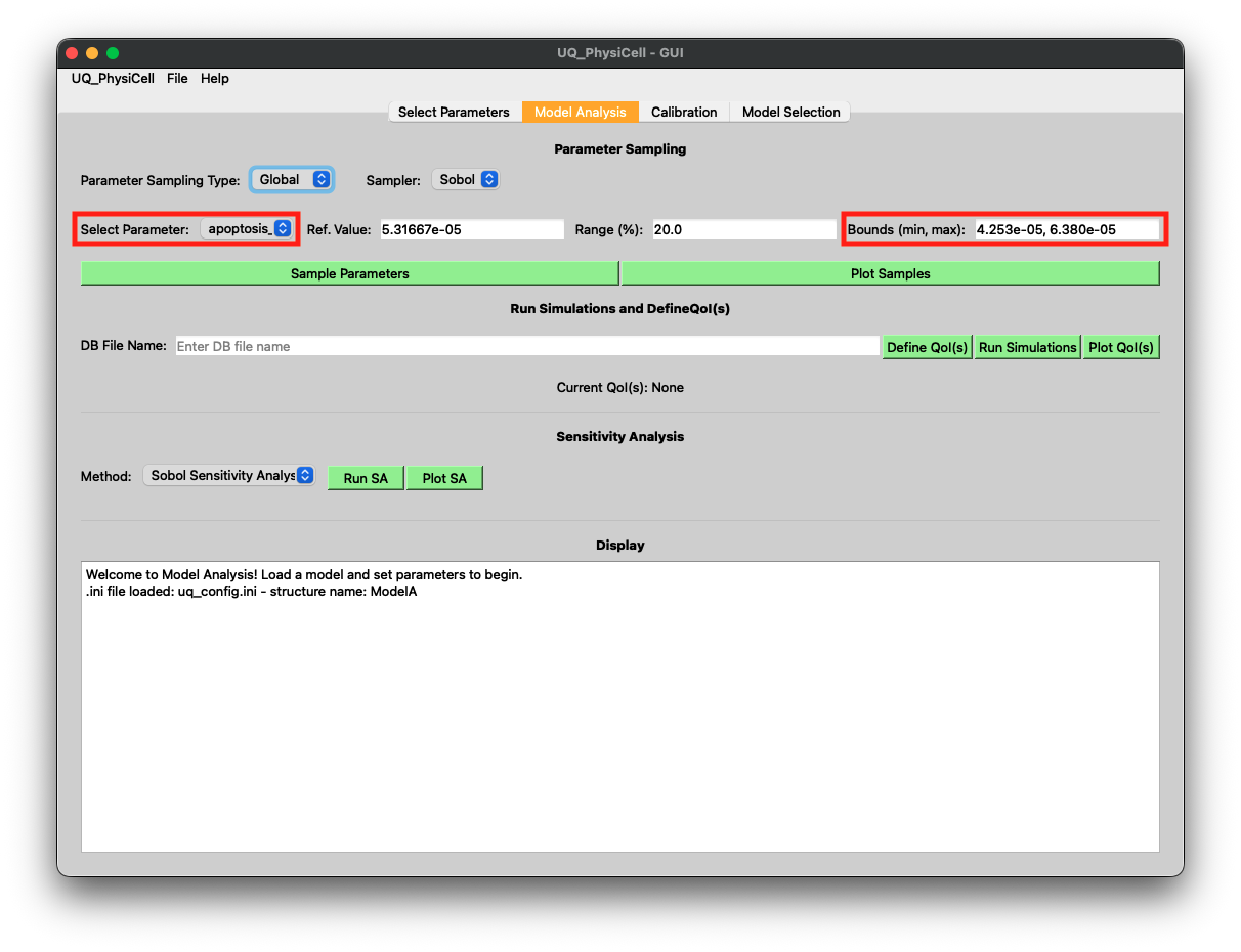
Left: Define the parameter sampling strategy as `Global` (step 1). Right: Check the range of the `apoptosis_rate` parameter (step 2).
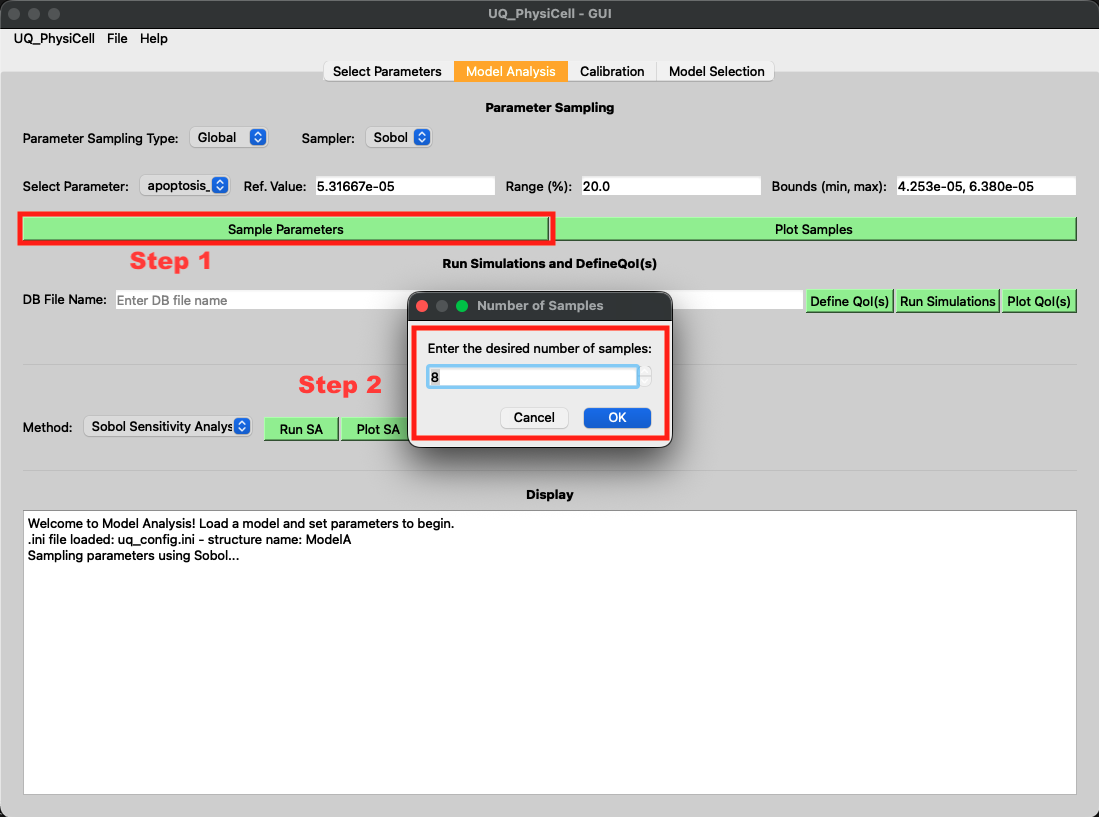
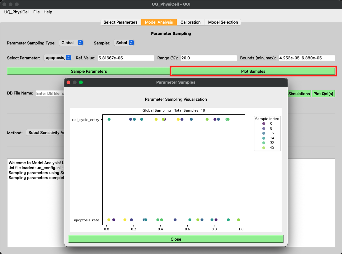
Left: Sample the parameters using Sobol sampling with 8 samples (step 3). Right: Plot the sampled parameters (step 3).
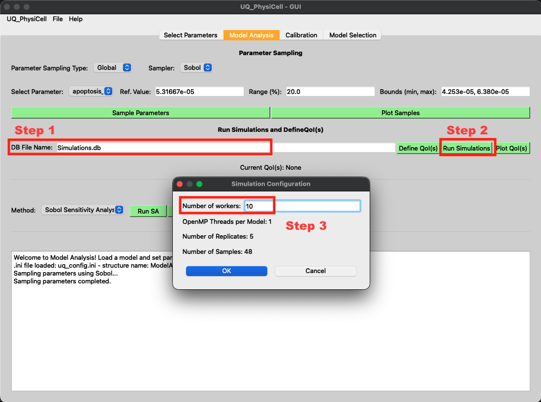
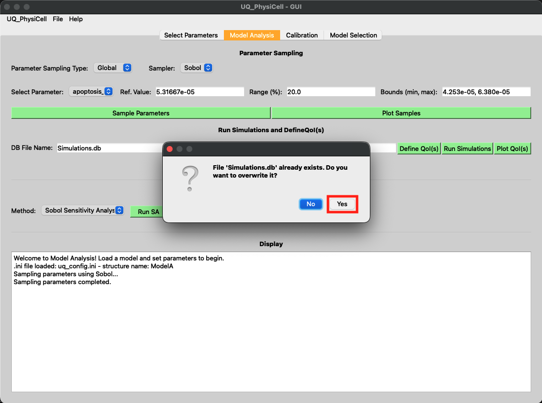
Left: Set the database filename as `Simulations.db`, click the Run Simulations button, and set the number of workers (step 4-5). Right: Confirm the storage of the MCDS objects list (step 5).
Step 4: Define Quantities of Interest (QoIs) and Perform Sensitivity Analysis
Finally, we’ll define the outputs we want to analyze and compute sensitivity indices to understand which parameters most influence the model behavior.
Steps:
Define the QoIs using the predefined options:
live_cellsanddead_cellsVisualize the mean values of the QoIs across all simulations
Run the sensitivity analysis and plot the results
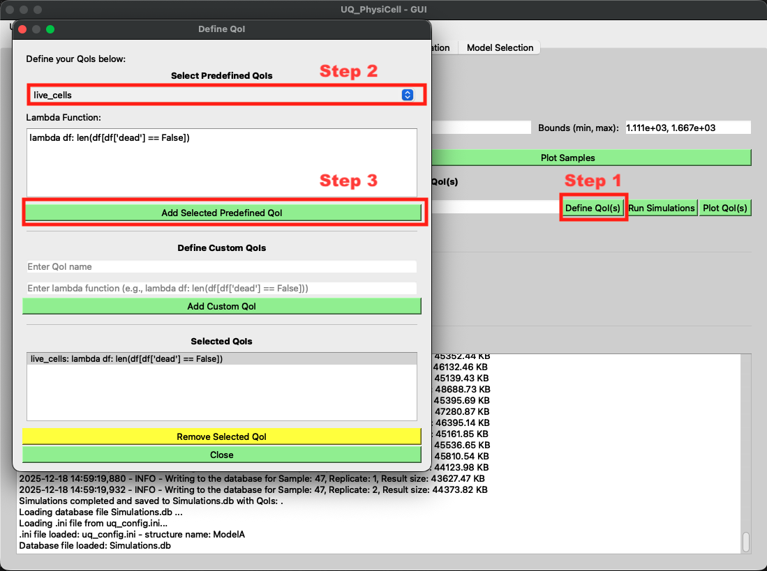
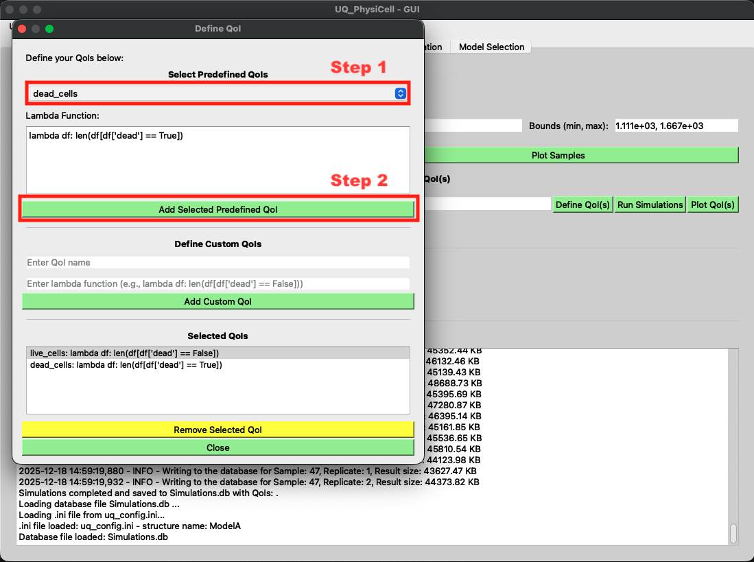
Left: Select `live_cells` QoI (step 1). Right: Select `dead_cells` QoI (step 1).
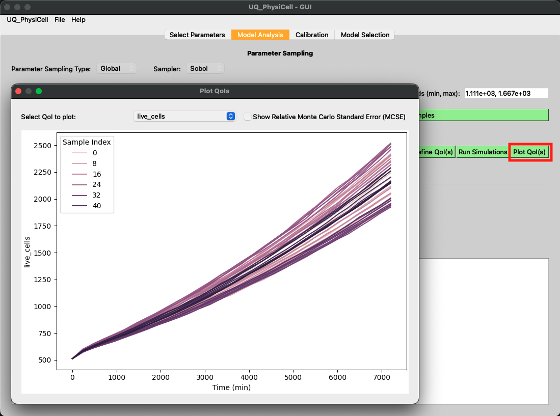
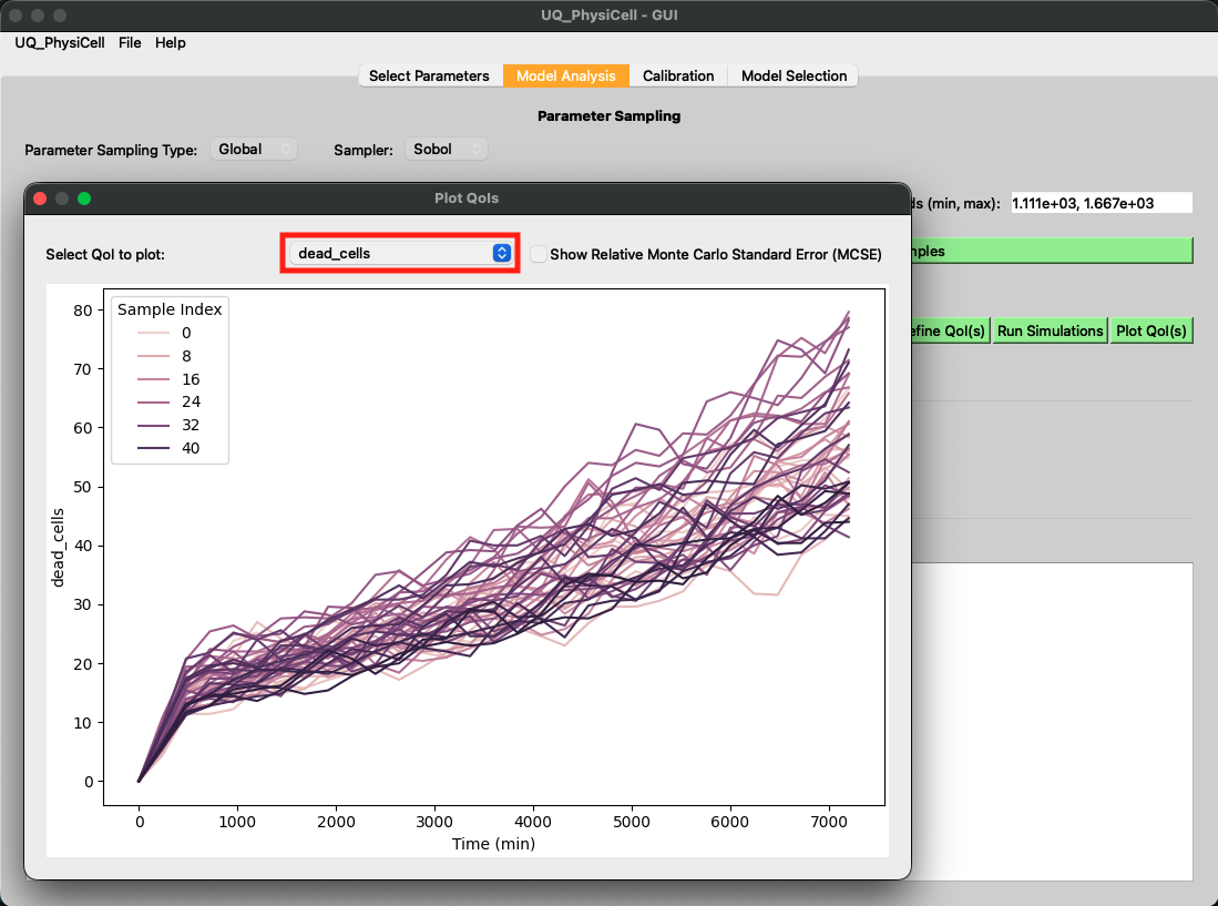
Left: Plot the QoIs (step 2). Right: Visualize the `dead_cells` QoI time series (step 2).
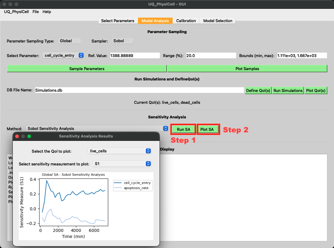
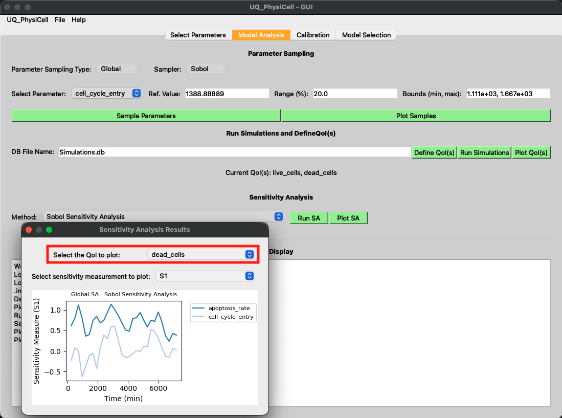
Left: Run and plot the sensitivity analysis (step 3). Right: Visualize the sensitivity indices for `dead_cells` (step 3).
Note
These QoIs were selected for demonstration purposes. Feel free to explore other predefined QoIs or create your own custom QoI. Note that other sensitivity analysis methods are also compatible with the Sobol sampling strategy, so you can experiment with different SA approaches as well.