Example 8: Model Calibration — Approximate Bayesian Computation (ABC-SMC)

(GitHub link)

This notebook calibrates the virus-mac-new model using ABC-SMC (Approximate Bayesian Computation — Sequential Monte Carlo). Unlike BO (ex7) which finds point estimates, ABC-SMC returns a full posterior distribution over parameters, quantifying how uncertain we are about each parameter given the observed data.

BO (ex7) vs ABC-SMC (ex8):

	Bayesian Optimization (ex7)	ABC-SMC (ex8)
Output	Pareto front (point estimates)	Posterior distribution
Tells you	Best-fit parameter values	Full uncertainty over parameters
Requires	Acquisition function + GP	Prior distribution + distance function
Best for	Finding optimal parameters	Uncertainty quantification

What you will learn:

• How to define prior distributions using pyABC’s Distribution and RV

• How distance functions replace the objective function from BO

• How ABC-SMC progressively tightens the tolerance (epsilon) across populations

• How to read the posterior: width reflects identifiability, coverage of the true value reflects accuracy

Ground truth (same observed data as ex7):

• mac_phag_rate_infected = 1.0

• epi2infected_hfm = 0.4

import warnings, logging
import numpy as np
import matplotlib.pyplot as plt
warnings.filterwarnings('ignore')

from uq_physicell.abc import CalibrationContext, run_abc_calibration
from pyabc import RV, Distribution, visualization

logging.basicConfig(level=logging.INFO)
logger = logging.getLogger(__name__)

db_path = "ex8_ABC_Calib.db"
obs_data_path = "ex7_ObsData.csv"
dic_real_value = {"mac_phag_rate_infected": 1.0, "epi2infected_hfm": 0.4}

model_config = {"ini_path": "uq_pc_struc.ini", "struc_name": "Model_struc_Calib"}

# df_cell → cell DataFrame (see ex1 for the full dispatch table)
qoi_functions = {
    "epi_":         lambda df_cell: len(df_cell[df_cell['cell_type'] == 'epithelial']),
    "epi_infected": lambda df_cell: len(df_cell[df_cell['cell_type'] == 'epithelial_infected']),
}

obs_data_columns = {
    "time":         "Time",
    "epi_":         "Healthy Epithelial Cells",
    "epi_infected": "Infected Epithelial Cells",
}

Distance functions, prior, and ABC options

def euclidean_distance_epi(data1, data2):
    obs_vals = np.array(data1['epi_'])
    sim_vals = np.array(data2['epi_'])
    return np.sum((obs_vals - sim_vals) ** 2)

def euclidean_distance_epi_infected(data1, data2):
    obs_vals = np.array(data1['epi_infected'])
    sim_vals = np.array(data2['epi_infected'])
    return np.sum((obs_vals - sim_vals) ** 2)

distance_functions = {
    "epi_":         {"function": euclidean_distance_epi},
    "epi_infected": {"function": euclidean_distance_epi_infected},
}

# Uniform priors over the same bounds as ex7 for direct comparison
prior = Distribution(
    mac_phag_rate_infected=RV("uniform", 0.7, 0.8),   # uniform on [0.7, 1.5]
    epi2infected_hfm=RV("uniform", 0.1, 0.4),          # uniform on [0.1, 0.5]
)

abc_options = {
    "max_populations": 2,
    "max_simulations": 100,
    "population_strategy": "adaptive",
    "min_population_size": 10,
    "max_population_size": 50,
    "adaptive_distance": True,
    "sampler": "multicore",
    "num_workers": 6,
}

Create context and run ABC-SMC calibration

calib_context = CalibrationContext(
    db_path=db_path,
    obsData=obs_data_path,
    obsData_columns=obs_data_columns,
    model_config=model_config,
    qoi_functions=qoi_functions,
    distance_functions=distance_functions,
    prior=prior,
    abc_options=abc_options,
    logger=logger,
)

history = run_abc_calibration(calib_context=calib_context)
print(f"Completed — {history.n_populations} populations, {history.total_nr_simulations} total simulations")

ABC.Sampler INFO: Parallelize sampling on 1 processes.
INFO:ABC.Sampler:Parallelize sampling on 1 processes.

Completed — 1 populations, 158 total simulations

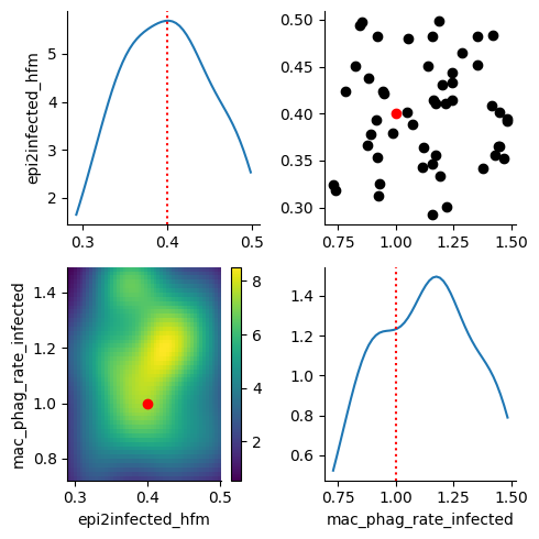
Posterior analysis

The posterior distribution shows how much each parameter value is supported by the observed data. A narrow posterior means the data is informative about that parameter; a wide posterior means it is hard to identify from this QoI alone.

if history.n_populations > 1:
    fig, ax = plt.subplots(figsize=(8, 5))
    visualization.plot_epsilons(history, yscale='linear', ax=ax)
    ax.set_title("Tolerance (epsilon) over ABC-SMC populations")

df_posterior, w = history.get_distribution(m=0, t=history.max_t)
display(df_posterior.head())

print("\nParameter recovery:")
for param, true_val in dic_real_value.items():
    mean = df_posterior[param].mean()
    std  = df_posterior[param].std()
    print(f"  {param}: true={true_val:.3f}  posterior={mean:.3f} ± {std:.3f}  (relative error {abs(mean-true_val)/true_val*100:.1f}%)")

visualization.plot_kde_matrix(df_posterior, w, refval=dic_real_value, refval_color="red")

name	epi2infected_hfm	mac_phag_rate_infected
id
2	0.346153	1.159550
3	0.354043	0.920385
4	0.401899	1.447023
5	0.451707	1.355795
6	0.366163	0.875740

Parameter recovery:
  mac_phag_rate_infected: true=1.000  posterior=1.132 ± 0.220  (relative error 13.2%)
  epi2infected_hfm: true=0.400  posterior=0.401 ± 0.057  (relative error 0.2%)

array([[<Axes: ylabel='epi2infected_hfm'>, <Axes: >],
       [<Axes: xlabel='epi2infected_hfm', ylabel='mac_phag_rate_infected'>,
        <Axes: xlabel='mac_phag_rate_infected'>]], dtype=object)

---

This completes the UQ-PhysiCell example series. To combine sampling (ex5/ex6) with calibration (ex7/ex8), use calculate_qoi_from_db_file to compute QoIs from an existing raw-MCDS database and feed them into a CalibrationContext without re-running any simulations.