Example 10: Rule Inactivation Sensitivity Analysis — Pancreatic Cancer Invasion Model

(GitHub link)

This notebook presents a custom sensitivity analysis of rule inactivation in the model developed in Johnson et al. 2025, which represents pancreatic cancer invasion mediated by fibroblast-ECM interactions. The analysis uses an OAT-style perturbation: starting from the nominal model (all rules active), one rule is inactivated at a time, and the deviation in model outputs relative to the full model is quantified using RMSD.

What you will learn:

• How to encode categorical/rule-based perturbations as samples in a ModelAnalysisContext database

• How to use load_samples and calculate_qoi_statistics on a raw-MCDS database (Mode B from ex2)

• How to compute and normalize RMSD across multiple initial conditions for interpretable rule ranking

• How to visualize cell spatial distributions with plot_cells_2D

Rules analyzed (one inactivated at a time):

Rule	Description
Epi. Normal CIP	Contact inhibition of proliferation in normal epithelial cells
EMT Normal cell	Epithelial-to-mesenchymal transition in normal epithelial cells
MET Normal cell	Inhibition of mesenchymal-to-epithelial transition in normal mesenchymal cells
Slow/Speed up N-MC	Motility modulation of normal mesenchymal cells
Slow/Speed up CAF	Motility modulation of cancer-associated fibroblasts
Epi. Tumor CIP	Contact inhibition of proliferation in epithelial tumor cells
EMT/MET Tumor cell	EMT and MET transitions in tumor cells
Slow/Speed up TA-MC	Motility modulation of tumor-associated mesenchymal cells

Simulations were run across 7 initial conditions (epithelial tumor cell-to-CAF seeding ratios with 1,000 total cells), simulated for 7 days with multiple stochastic replicates.

from uq_physicell.model_analysis import calculate_qoi_statistics

db_file = 'uq_Simulations_OAT_CoCulture.db'

# df_cell → cell DataFrame (see ex1 for the full dispatch table)
qoi_funcs = {
    'epi_normal_cell_count':    lambda df_cell: len(df_cell[(df_cell['dead'] == False) & (df_cell['cell_type'] == 'epithelial_normal')]),
    'mesenc_normal_cell_count': lambda df_cell: len(df_cell[(df_cell['dead'] == False) & (df_cell['cell_type'] == 'mesenchymal_normal')]),
    'fibroblast_cell_count':    lambda df_cell: len(df_cell[(df_cell['dead'] == False) & (df_cell['cell_type'] == 'fibroblast')]),
    'epi_tumor_cell_count':     lambda df_cell: len(df_cell[(df_cell['dead'] == False) & (df_cell['cell_type'] == 'epithelial_tumor')]),
    'mesenc_tumor_cell_count':  lambda df_cell: len(df_cell[(df_cell['dead'] == False) & (df_cell['cell_type'] == 'mesenchymal_tumor')]),
    'epi_normal_radial_dist':   lambda df_cell: df_cell[df_cell['cell_type'] == 'epithelial_normal'][['position_x','position_y','position_z']].apply(lambda r: (r**2).sum()**0.5, axis=1).mean(),
    'mesenc_normal_radial_dist':lambda df_cell: df_cell[df_cell['cell_type'] == 'mesenchymal_normal'][['position_x','position_y','position_z']].apply(lambda r: (r**2).sum()**0.5, axis=1).mean(),
    'fibroblast_radial_dist':   lambda df_cell: df_cell[df_cell['cell_type'] == 'fibroblast'][['position_x','position_y','position_z']].apply(lambda r: (r**2).sum()**0.5, axis=1).mean(),
    'epi_tumor_radial_dist':    lambda df_cell: df_cell[df_cell['cell_type'] == 'epithelial_tumor'][['position_x','position_y','position_z']].apply(lambda r: (r**2).sum()**0.5, axis=1).mean(),
    'mesenc_tumor_radial_dist': lambda df_cell: df_cell[df_cell['cell_type'] == 'mesenchymal_tumor'][['position_x','position_y','position_z']].apply(lambda r: (r**2).sum()**0.5, axis=1).mean(),
}

# ignore_db_consistency=True because 2 samples are missing from the Output table
df_summary_mean, df_summary_std, df_summary_mcse = calculate_qoi_statistics(db_file, qoi_funcs, ignore_db_consistency=True)
display(df_summary_mean)

No QoI data provided, calculating QoIs from the database...
2 from Samples table is missing in Output table.
 Missing SampleIDs: [61, 62]
Warning: Database consistency check failed, but proceeding as per user request.
Calculating QoIs from mcds list...

		epi_normal_cell_count	epi_normal_radial_dist	epi_tumor_cell_count	epi_tumor_radial_dist	fibroblast_cell_count	fibroblast_radial_dist	mesenc_normal_cell_count	mesenc_normal_radial_dist	mesenc_tumor_cell_count	mesenc_tumor_radial_dist
SampleID	time
0	0.0	0.0	NaN	500.0	192.045556	500.0	183.661279	0.0	NaN	0.0	NaN
	1440.0	0.0	NaN	35.6	283.491670	500.0	195.036377	0.0	NaN	544.6	205.741238
	2880.0	0.0	NaN	49.4	330.193621	500.0	203.653420	0.0	NaN	567.8	218.598059
	4320.0	0.0	NaN	90.8	354.745680	500.0	211.526886	0.0	NaN	586.6	230.352639
	5760.0	0.0	NaN	150.0	379.339727	500.0	218.391999	0.0	NaN	618.6	242.760217
...	...	...	...	...	...	...	...	...	...	...	...
90	4320.0	0.0	NaN	2126.6	279.996736	90.0	218.673131	0.0	NaN	317.0	231.617323
	5760.0	0.0	NaN	2687.0	313.017651	90.0	223.993993	0.0	NaN	374.4	249.552555
	7200.0	0.0	NaN	3342.4	346.349592	90.0	229.256590	0.0	NaN	404.0	255.734771
	8640.0	0.0	NaN	4084.4	379.990875	90.0	231.584211	0.0	NaN	435.0	257.400322
	10080.0	0.0	NaN	4896.0	413.570264	90.0	233.510260	0.0	NaN	482.4	265.475861

712 rows × 10 columns

Map sample IDs to rules and initial conditions

from uq_physicell.model_analysis import load_samples
import pandas as pd

# Normalize the QOIs by the nominal case (row with all rules activated)
dic_parameters = load_samples(db_file)
df_samples_desc = pd.DataFrame.from_dict(dic_parameters, orient='index')
df_samples_desc.index.name = 'SampleID'
df_samples_desc['Inactive_rule'] = df_samples_desc.apply(
    lambda row: next((key for key, value in row.items() if key != 'IC_file' and value == 1), None),
    axis=1
)
# Drop the original parameter columns, keeping only 'IC_file' and 'Inactive_rule'
df_samples_desc = df_samples_desc[['IC_file', 'Inactive_rule']]
dic_rules_names = { 'epi_normal_rule_pressureDcellcycle_inactive': 'Epi. Normal CIP', # Contact inhibition of proliferation in normal epithelial cells
                   'epi_normal_rule_ecmImesenc_normal_inactive': 'EMT Normal cell', # Transition from epithelial to mesenchymal state (EMT) in normal epithelial cells
                   'mesenc_normal_rule_ecmDspeed_inactive': 'Slow down N-MC', # Slow down normal mesenchymal cells (N-MC) by decreasing their speed
                   'mesenc_normal_rule_ecmIspeed_inactive': 'Speed up N-MC', # Speed up normal mesenchymal cells (N-MC) by increasing their speed
                   'mesenc_normal_rule_infsignalDepi_normal_inactive': 'MET Normal cell', # Inhibition of transition from mesenchymal state to epithelial (MET) in normal mesenchymal cells (N-MC)
                   'fib_rule_ecmDspeed_inactive': 'Slow down CAF', # Slow down cancer-associated fibroblasts (CAF) by decreasing their speed
                   'fib_rule_ecmIspeed_inactive': 'Speed up CAF', # Speed up cancer-associated fibroblasts (CAF) by increasing their speed
                   'epi_tumor_rule_pressureDcellcycle_inactive': 'Epi. Tumor CIP', # Contact inhibition of proliferation in tumor epithelial cells
                   'epi_tumor_rule_ecmImesenc_tumor_inactive': 'EMT Tumor cell', # Transition from epithelial to mesenchymal state (EMT) in tumor epithelial cells
                   'mesenc_tumor_rule_ecmDspeed_inactive': 'Slow down TA-MC', # Slow down tumor associated mesenchymal cells (TA-MC) by decreasing their speed
                   'mesenc_tumor_rule_ecmIspeed_inactive': 'Speed up TA-MC', # Speed up tumor associated mesenchymal cells (TA-MC) by increasing their speed
                   'mesenc_tumor_rule_infsignalDepi_tumor_inactive': 'MET Tumor cell', # Inhibition of transition from mesenchymal state to epithelial (MET) in tumor mesenchymal cells
                    }
# Rename the Inactive_rule values based on the dic_rules_names mapping
df_samples_desc['Inactive_rule'] = df_samples_desc['Inactive_rule'].map(dic_rules_names).fillna(df_samples_desc['Inactive_rule'])
display(df_samples_desc)

	IC_file	Inactive_rule
SampleID
0	cells_1_to_1.csv	None
1	cells_1_to_2.csv	None
2	cells_1_to_5.csv	None
3	cells_1_to_10.csv	None
4	cells_2_to_1.csv	None
...	...	...
86	cells_1_to_5.csv	MET Tumor cell
87	cells_1_to_10.csv	MET Tumor cell
88	cells_2_to_1.csv	MET Tumor cell
89	cells_5_to_1.csv	MET Tumor cell
90	cells_10_to_1.csv	MET Tumor cell

91 rows × 2 columns

import matplotlib.pyplot as plt
import seaborn as sns

# Define color palette for different initial conditions
palette = sns.color_palette("colorblind")
my_palette = {}
for ic in df_samples_desc['IC_file'].unique():
    my_palette[ic] = palette[len(my_palette) % len(palette)]
# Make sure 'time' is a column in df_summary_mean for plotting
df_summary_mean_ = df_summary_mean.reset_index('time')
# Include the mapping of SampleID to IC_file in df_summary_mean for plotting
df_summary_mean_["IC_file"] = df_summary_mean_.index.map(df_samples_desc['IC_file'])
qois_with_changes = [ col for col in qoi_funcs.keys() if (df_summary_mean_[col].max() != df_summary_mean_[col].min()) and (col != 'time') and not pd.isnull(df_summary_mean_[col].max()) ]  # Identify QoIs that have changes across samples (exclude time column)
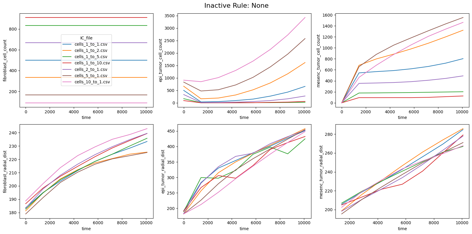
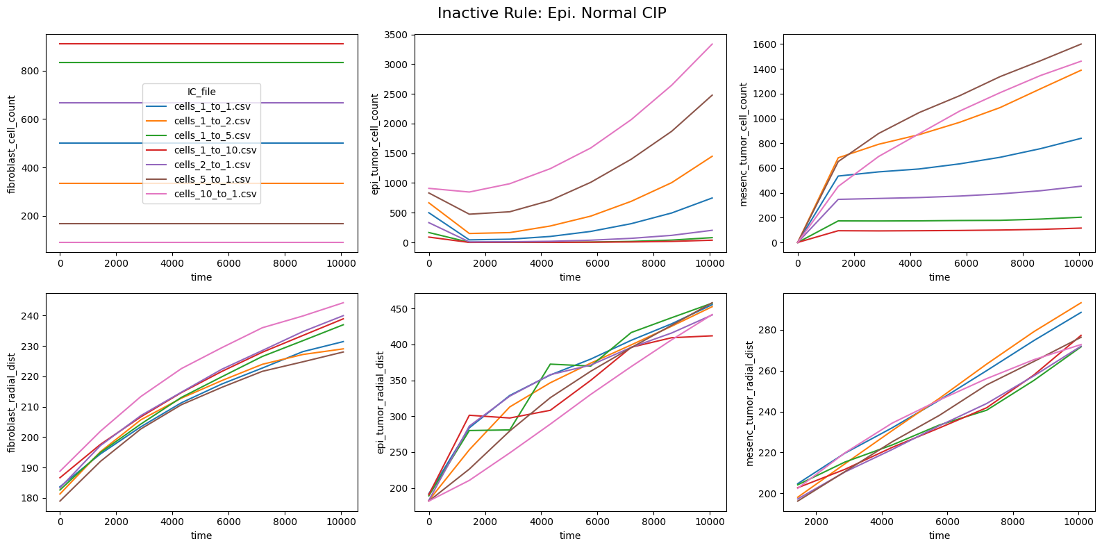
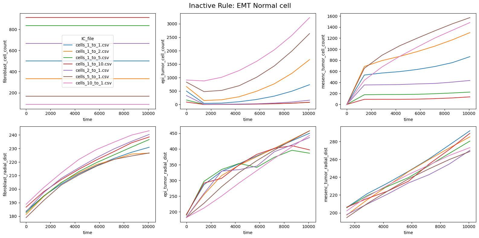
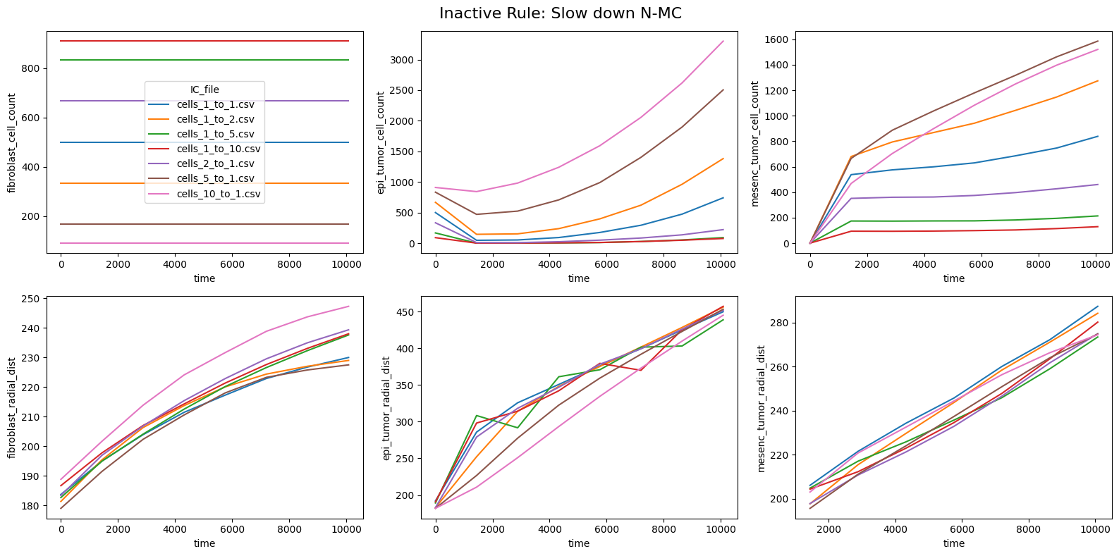
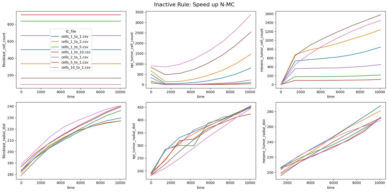
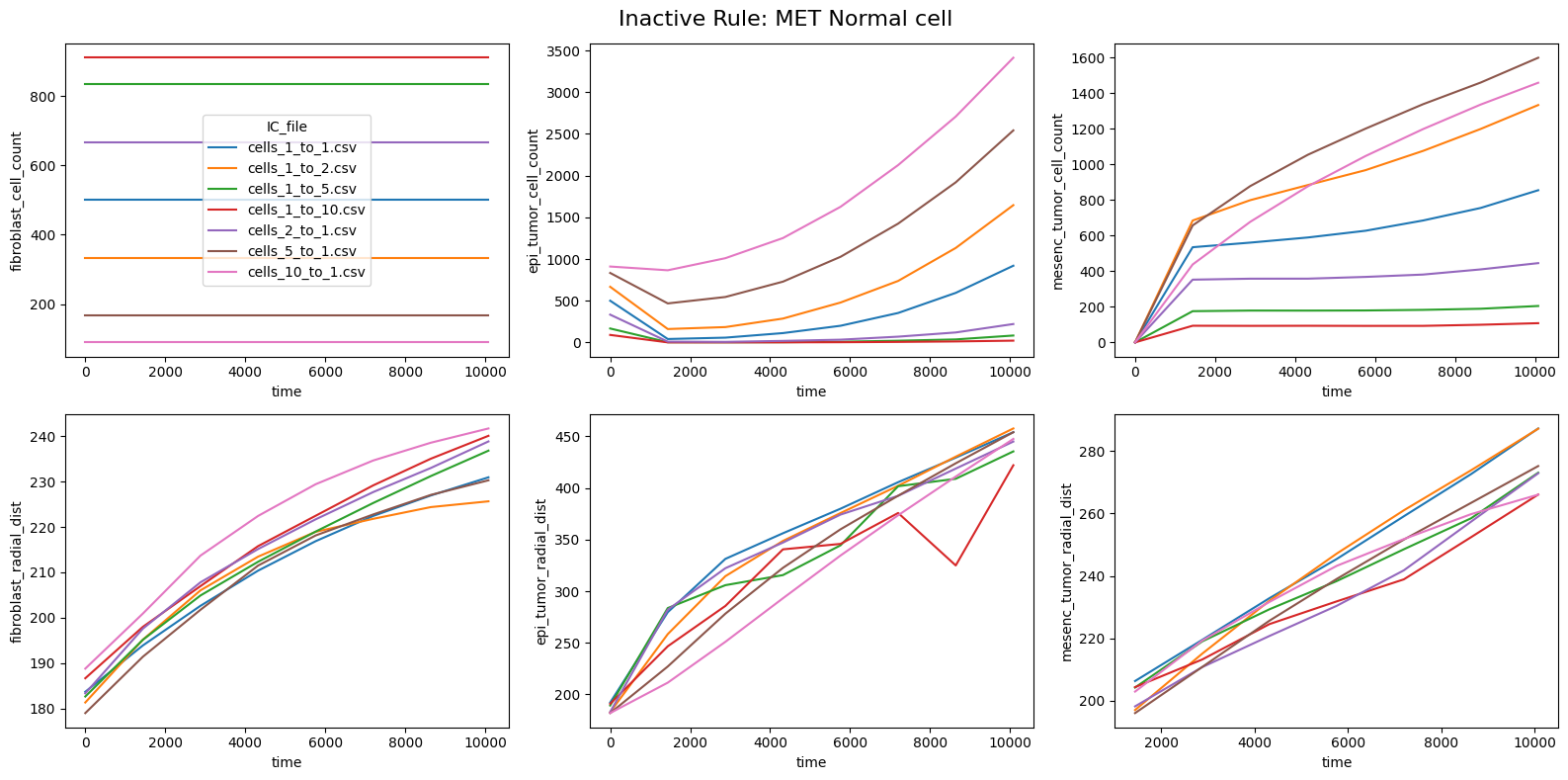
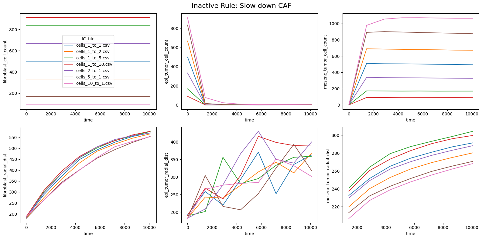
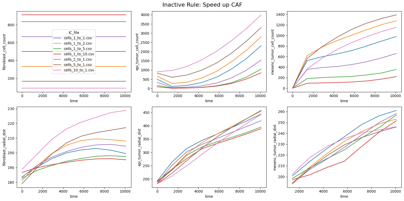
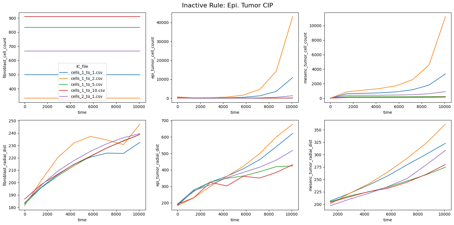
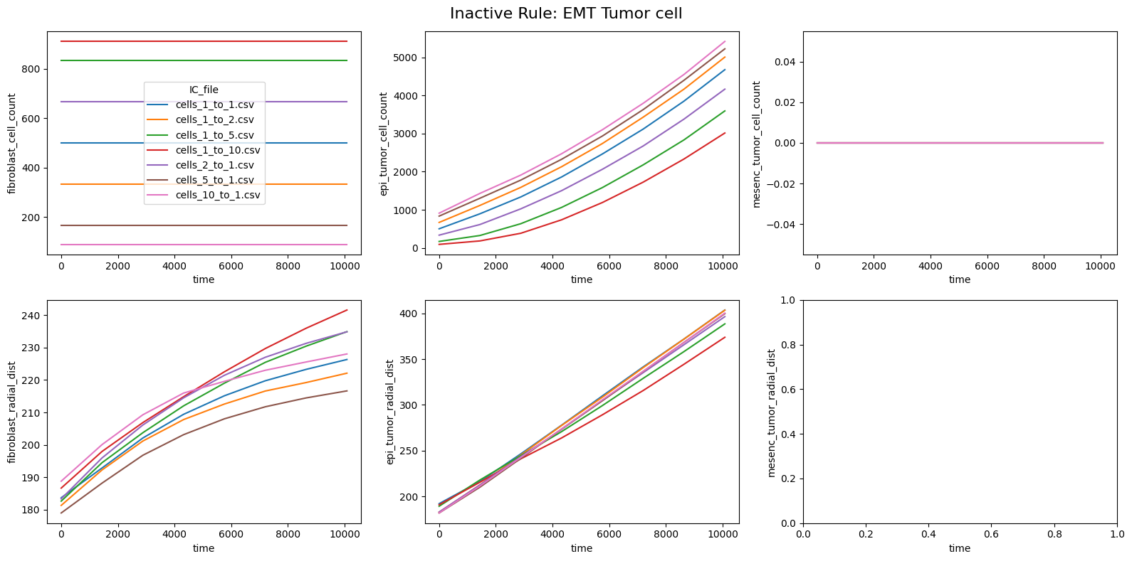
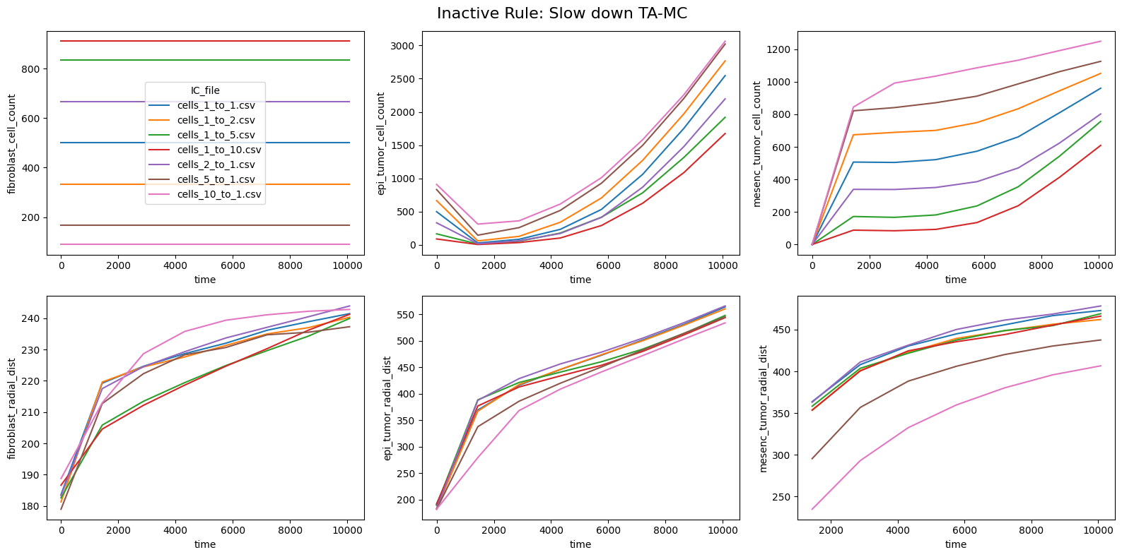
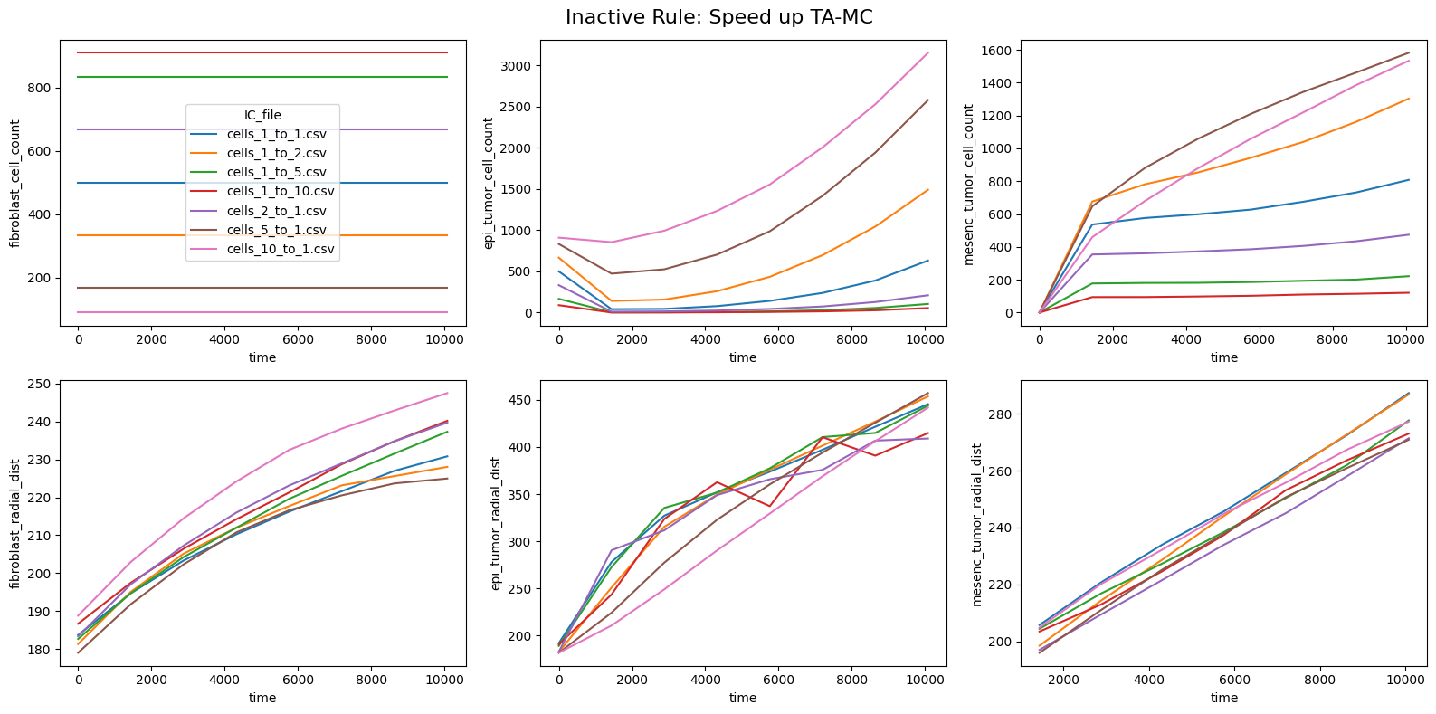
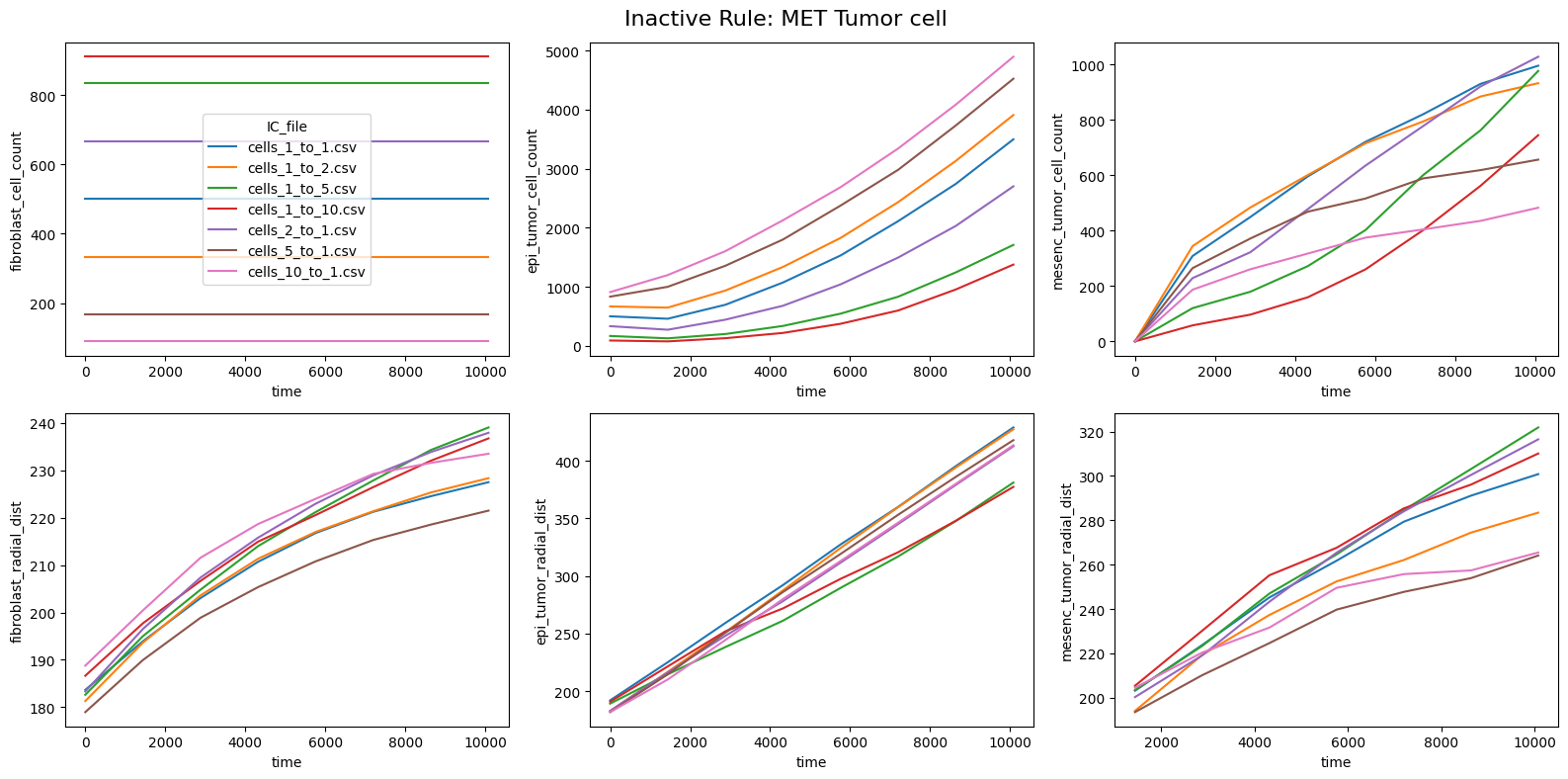
for inac_rule in df_samples_desc['Inactive_rule'].unique():
    fig, axes = plt.subplots(2,3,figsize=(16, 8))
    axes_f = axes.flatten()
    fig.suptitle(f'Inactive Rule: {inac_rule}', fontsize=16)
    if inac_rule is None: df_summary_qois_plot = df_summary_mean_.loc[df_samples_desc['Inactive_rule'].isna()].reset_index()  # Filter for the nominal case (all rules active)
    else: df_summary_qois_plot = df_summary_mean_.loc[df_samples_desc['Inactive_rule'] == inac_rule].reset_index()  # Filter for inactive rule
    for id_qoi, qoi in enumerate(qois_with_changes):
        sns.lineplot(data=df_summary_qois_plot, x="time", y=qoi, hue="IC_file", ax=axes_f[id_qoi], legend=True if id_qoi==0 else False)
    fig.tight_layout()
    plt.savefig(f'CoCulture_QoIs_{inac_rule}.svg', format='svg')

Compute RMSD relative to the nominal (all-rules-active) model

import pandas as pd
import numpy as np

# Use SampleID as the main index; time stays as a column for alignment within each sample
qoi_cols = list(qoi_funcs.keys())
df_rmsd = pd.DataFrame(index=df_samples_desc.index, columns=qoi_cols, dtype=float)
for ic_file in df_samples_desc['IC_file'].unique():
    sampleids = df_samples_desc.index[df_samples_desc['IC_file'] == ic_file].tolist()
    nominal_sampleid = df_samples_desc.index[(df_samples_desc['IC_file'] == ic_file) & (df_samples_desc['Inactive_rule'].isna())].tolist()[0]  # SampleID for the nominal case (all rules active)
    samples_missing = [sid for sid in sampleids if sid not in df_summary_mean_.index]
    samples_present = [sid for sid in sampleids if sid in df_summary_mean_.index]
    print(f"Taking the squared difference of IC_file: {ic_file} with nominal SampleID: {nominal_sampleid}. Samples missing: {samples_missing}")

    nominal_qois = df_summary_mean_.loc[nominal_sampleid, ['time'] + qoi_cols].set_index('time')
    for sid in samples_present:
        current_qois = df_summary_mean_.loc[sid, ['time'] + qoi_cols].set_index('time')
        common_time = current_qois.index.intersection(nominal_qois.index)
        if len(common_time) == 0:
            continue
        df_rmsd.loc[sid, qoi_cols] = np.sqrt(((current_qois.loc[common_time, qoi_cols] - nominal_qois.loc[common_time, qoi_cols]) ** 2).mean())

df_rmsd = df_rmsd.fillna(0)  # Fill NaN values with 0 for samples that are missing (since we cannot calculate RMSD without data, we set it to 0 to indicate no deviation from nominal)
display("RMSD: ", df_rmsd)

Taking the squared difference of IC_file: cells_1_to_1.csv with nominal SampleID: 0. Samples missing: []
Taking the squared difference of IC_file: cells_1_to_2.csv with nominal SampleID: 1. Samples missing: []
Taking the squared difference of IC_file: cells_1_to_5.csv with nominal SampleID: 2. Samples missing: []
Taking the squared difference of IC_file: cells_1_to_10.csv with nominal SampleID: 3. Samples missing: []
Taking the squared difference of IC_file: cells_2_to_1.csv with nominal SampleID: 4. Samples missing: []
Taking the squared difference of IC_file: cells_5_to_1.csv with nominal SampleID: 5. Samples missing: [61]
Taking the squared difference of IC_file: cells_10_to_1.csv with nominal SampleID: 6. Samples missing: [62]

'RMSD: '

	epi_normal_cell_count	mesenc_normal_cell_count	fibroblast_cell_count	epi_tumor_cell_count	mesenc_tumor_cell_count	epi_normal_radial_dist	mesenc_normal_radial_dist	fibroblast_radial_dist	epi_tumor_radial_dist	mesenc_tumor_radial_dist
SampleID
0	0.0	0.0	0.0	0.000000	0.000000	0.0	0.0	0.000000	0.000000	0.000000
1	0.0	0.0	0.0	0.000000	0.000000	0.0	0.0	0.000000	0.000000	0.000000
2	0.0	0.0	0.0	0.000000	0.000000	0.0	0.0	0.000000	0.000000	0.000000
3	0.0	0.0	0.0	0.000000	0.000000	0.0	0.0	0.000000	0.000000	0.000000
4	0.0	0.0	0.0	0.000000	0.000000	0.0	0.0	0.000000	0.000000	0.000000
...	...	...	...	...	...	...	...	...	...	...
86	0.0	0.0	0.0	828.170426	378.092733	0.0	0.0	2.683751	62.263029	31.207755
87	0.0	0.0	0.0	626.444774	297.970057	0.0	0.0	1.496992	49.312425	32.315537
88	0.0	0.0	0.0	1275.408850	304.361348	0.0	0.0	0.858326	63.920350	28.567824
89	0.0	0.0	0.0	1287.343445	631.416400	0.0	0.0	3.967260	32.557048	3.908269
90	0.0	0.0	0.0	975.828130	658.141520	0.0	0.0	5.299893	22.378075	3.189457

91 rows × 10 columns

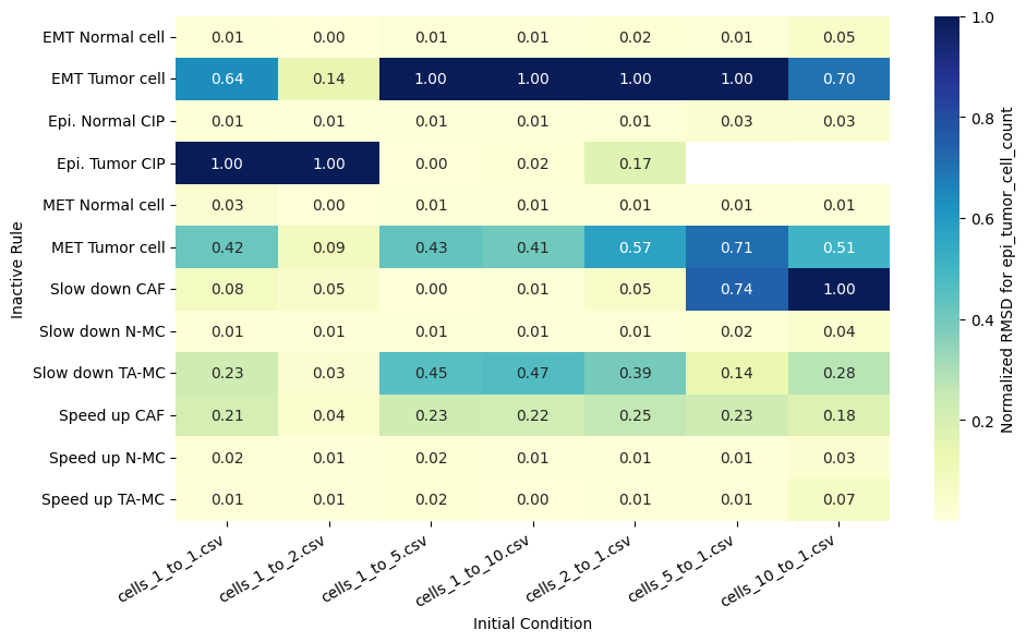
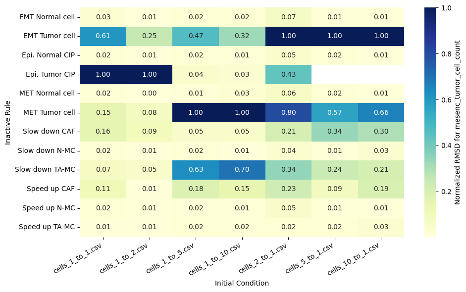
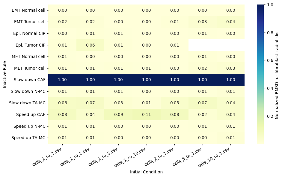
Normalize and plot RMSD per rule and initial condition

import seaborn as sns
import matplotlib.pyplot as plt

# Normalize per column and IC (each QOI independently for better visualization)
df_rmsd_normalized = pd.DataFrame(index=df_rmsd.index, columns=df_rmsd.columns, dtype=float)
for ic_file in df_samples_desc['IC_file'].unique():
    sampleids = df_samples_desc.index[df_samples_desc['IC_file'] == ic_file].tolist()
    samples_present = [sid for sid in sampleids if sid in df_summary_mean_.index]
    # Feature-wise normalization for the current IC (divide by the range of each column for the samples of the same IC) - Normalized RMSD (NRMSD)
    df_rmsd_normalized.loc[samples_present] = df_rmsd.loc[samples_present] / (df_rmsd.loc[samples_present].max(axis=0) - df_rmsd.loc[samples_present].min(axis=0))

# Remove columns with all NaN values
df_rmsd_normalized = df_rmsd_normalized.dropna(axis='columns', how='all')
# Replace NaN values (from zero-range normalization) with 0
valid_columns = df_rmsd_normalized.columns
print(f"Valid columns: {valid_columns}")

# Include IC_file and Inactive_rule for coloring and grouping in the plot
df_rmsd_normalized['IC_file'] = df_rmsd_normalized.index.map(df_samples_desc['IC_file'])
df_rmsd_normalized['Inactive_rule'] = df_rmsd_normalized.index.map(df_samples_desc['Inactive_rule'])

ic_order = list(my_palette.keys())

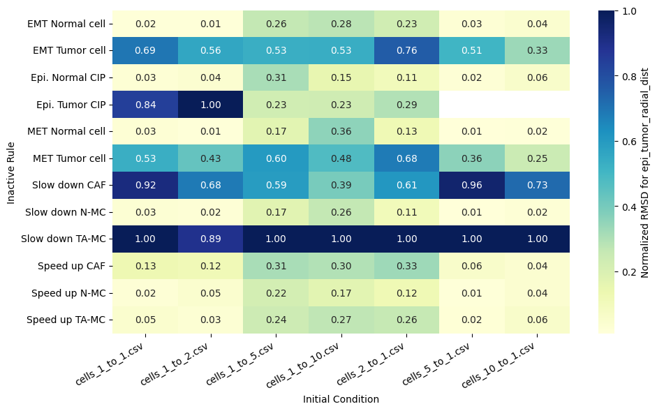
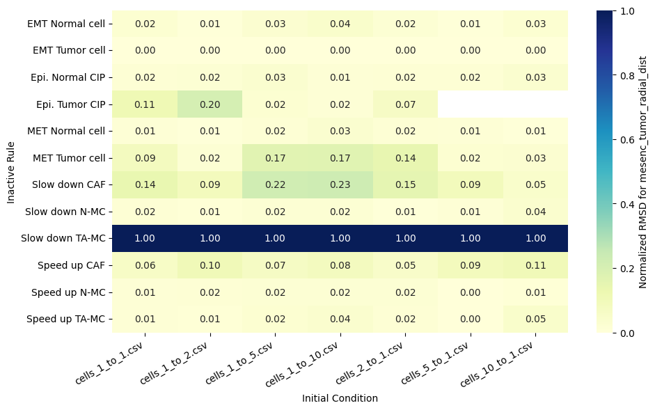
for qoi in valid_columns:
    fig, ax = plt.subplots(figsize=(10, 6))
    df_rmsd_normalized_plot = df_rmsd_normalized.sort_values(by=qoi, ascending=False)
    df_rmsd_normalized_plot = df_rmsd_normalized_plot[df_rmsd_normalized_plot['Inactive_rule'].notna()]
    # sns.boxplot(data=df_rmsd_normalized_plot, x=qoi, y="Inactive_rule", color="white", showfliers=False)
    # sns.swarmplot(data=df_rmsd_normalized_plot, x=qoi, y="Inactive_rule", hue="IC_file", color="0.25", size=6, palette=my_palette,  hue_order=my_palette.keys(), dodge=True)
    # plt.legend(title="Initial Condition", bbox_to_anchor=(1.05, 1), loc='upper left')
    # ax.set(xlabel=f'Normalized RMSD for {qoi}', ylabel='Inactive Rule')
    heatmap_data = df_rmsd_normalized_plot.pivot(index='Inactive_rule', columns='IC_file', values=qoi).reindex(columns=ic_order)
    sns.heatmap(heatmap_data, annot=True, fmt=".2f", cmap="YlGnBu", cbar_kws={'label': f'Normalized RMSD for {qoi}'}, ax=ax)
    ax.set(xlabel='Initial Condition', ylabel='Inactive Rule')
    ax.set_xticklabels(ax.get_xticklabels(), rotation=30, ha='right')
    plt.tight_layout()
    plt.savefig(f'CoCulture_NormalizedRMSD_{qoi}.svg', format='svg')

Valid columns: Index(['epi_tumor_cell_count', 'mesenc_tumor_cell_count',
       'fibroblast_radial_dist', 'epi_tumor_radial_dist',
       'mesenc_tumor_radial_dist'],
      dtype='object')

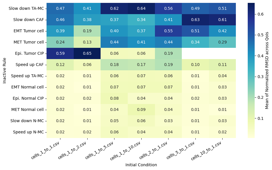
Rank rules by mean normalized RMSD across all QoIs

# Mean of normalized rmsd for all features per IC (take the mean across features for each sample)
df_mean_normalized_rmsd = df_rmsd_normalized[['IC_file', 'Inactive_rule']].copy()  # Start with a DataFrame containing IC_file and Inactive_rule
df_mean_normalized_rmsd["Mean of Normalized RMSD"] = 0.0
for ic in df_rmsd_normalized['IC_file'].unique():
    sampleids = df_rmsd_normalized.index[df_rmsd_normalized['IC_file'] == ic].tolist()
    df_mean_normalized_rmsd.loc[sampleids, "Mean of Normalized RMSD"] = df_rmsd_normalized.loc[sampleids, valid_columns].mean(axis=1)  # Take the mean across features for the current IC

# Define the ranking of rules based on the mean of normalized RMSD
df_ranked = pd.DataFrame(index=df_rmsd_normalized['Inactive_rule'].unique(), columns=['count', 'mean', 'std', 'min', '25%', '50%', '75%', 'max'])
for inac_rule in df_rmsd_normalized['Inactive_rule'].unique():
    df_ranked.loc[inac_rule] = df_mean_normalized_rmsd[df_mean_normalized_rmsd['Inactive_rule'] == inac_rule]['Mean of Normalized RMSD'].describe()
df_ranked = df_ranked.sort_values(by='mean', ascending=False)
display(df_ranked)

# Plot the mean of normalized RMSD across features for each sample, colored by IC and grouped by Inactive_rule
fig, ax = plt.subplots(figsize=(10, 6))
df_mean_normalized_rmsd = df_mean_normalized_rmsd.sort_values(by="Mean of Normalized RMSD", ascending=False)
df_mean_normalized_rmsd_plot = df_mean_normalized_rmsd[df_mean_normalized_rmsd['Inactive_rule'].notna()]  # Drop rows where Inactive_rule is None
# sns.boxplot(data=df_mean_normalized_rmsd, x='Mean of Normalized RMSD', y='Inactive_rule', color='white', showfliers=False)
# sns.swarmplot(data=df_mean_normalized_rmsd, x='Mean of Normalized RMSD', y='Inactive_rule', hue='IC_file', hue_order=my_palette.keys(), palette=my_palette, dodge=True)
# ax.set(xlabel='Mean of Normalized RMSD across features', ylabel='Inactive Rule')
# plt.legend(title="Initial Condition", bbox_to_anchor=(1.05, 1), loc='upper left')
heatmap_data = df_mean_normalized_rmsd_plot.pivot(index='Inactive_rule', columns='IC_file', values='Mean of Normalized RMSD').reindex(columns=ic_order, index=df_ranked[df_ranked.index.notna()].index)
sns.heatmap(heatmap_data, annot=True, fmt=".2f", cmap="YlGnBu", cbar_kws={'label': 'Mean of Normalized RMSD across QoIs'}, ax=ax)
ax.set(xlabel='Initial Condition', ylabel='Inactive Rule')
ax.set_xticklabels(ax.get_xticklabels(),rotation=30, ha='right') 
plt.tight_layout()
plt.savefig('CoCulture_MeanNormalizedRMSD.svg', format='svg')

	count	mean	std	min	25%	50%	75%	max
Slow down TA-MC	7.0	0.527242	0.082545	0.408277	0.480845	0.505388	0.589553	0.636236
Slow down CAF	7.0	0.456883	0.116993	0.337297	0.378724	0.405487	0.536223	0.625503
EMT Tumor cell	7.0	0.404619	0.114585	0.193522	0.380904	0.400342	0.461467	0.553727
MET Tumor cell	7.0	0.326916	0.117214	0.126188	0.26615	0.336219	0.426064	0.441575
Epi. Tumor CIP	5.0	0.312581	0.289664	0.060066	0.062364	0.193541	0.593677	0.65326
Speed up CAF	7.0	0.132195	0.047643	0.062193	0.104834	0.115819	0.173963	0.189761
Speed up TA-MC	7.0	0.038832	0.025087	0.010794	0.01431	0.043642	0.0616	0.065565
EMT Normal cell	7.0	0.03876	0.028981	0.006251	0.015048	0.028163	0.068062	0.070685
Epi. Normal CIP	7.0	0.032798	0.021349	0.015944	0.01766	0.027006	0.037389	0.076541
MET Normal cell	7.0	0.031857	0.028217	0.005544	0.011966	0.020032	0.044144	0.085203
Slow down N-MC	7.0	0.03058	0.018486	0.012479	0.01492	0.029858	0.040413	0.061054
Speed up N-MC	7.0	0.028895	0.017567	0.009904	0.016446	0.01918	0.042163	0.055963
None	0.0	NaN	NaN	NaN	NaN	NaN	NaN	NaN

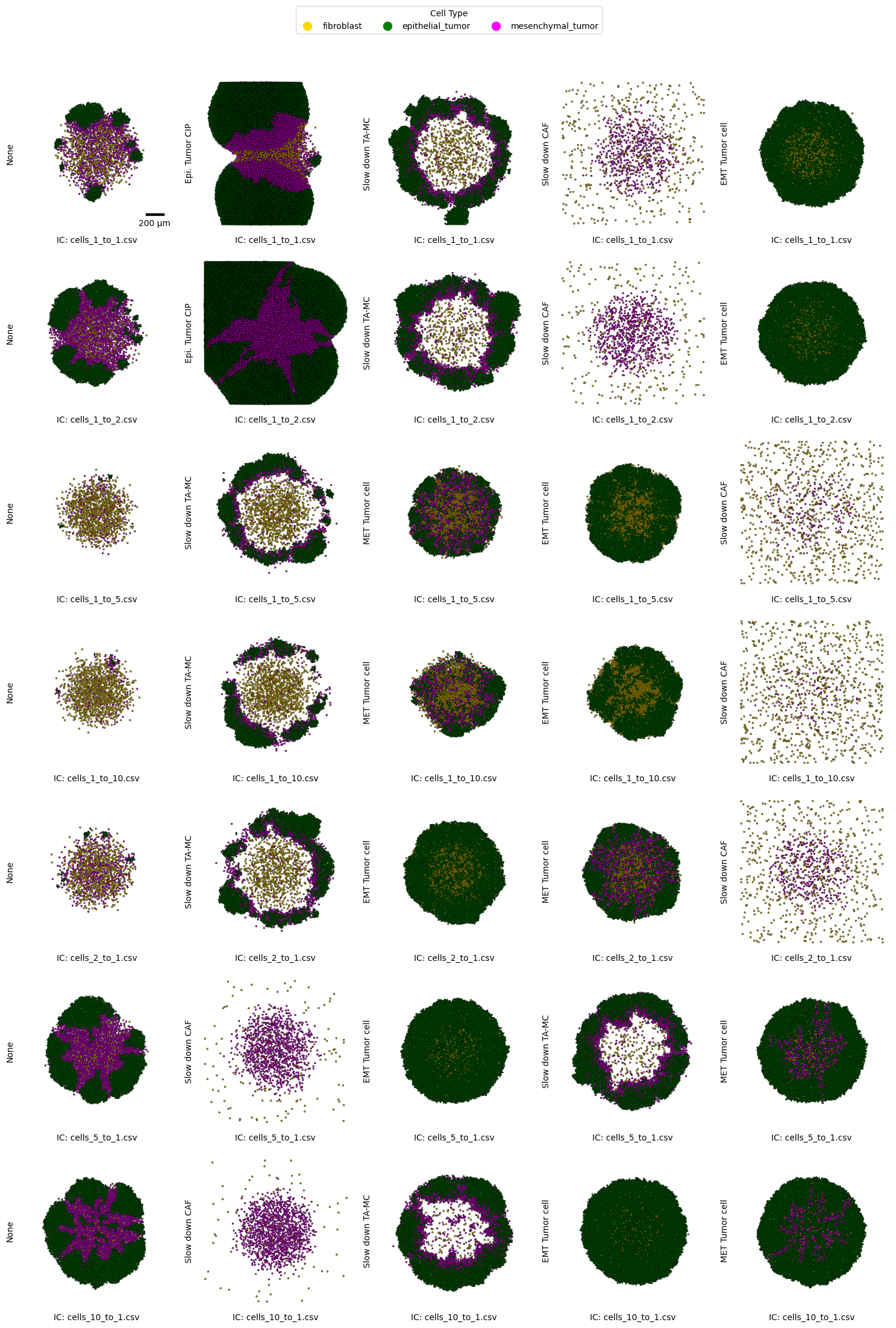
Cell snapshots — nominal vs top-sensitivity inactive rules

from uq_physicell.model_analysis import load_output, plot_cells_2D
from matplotlib.lines import Line2D

ICs = df_samples_desc['IC_file'].unique()
fig, axes = plt.subplots(len(ICs),5, figsize=(15, 3*len(ICs)), sharex=True, sharey=True)
max_labels = 0
color_dic = {'fibroblast': 'gold', 'epithelial_tumor': 'green', 'mesenchymal_tumor': 'magenta'}
particular_replicate_id = 0
for i, IC in enumerate(ICs):
    # First sample is the nominal case + top 4 max sensitivity inactive rules for the current IC
    top_samples_sensitivity = df_mean_normalized_rmsd.index[(df_mean_normalized_rmsd['IC_file'] == IC) & (df_mean_normalized_rmsd['Inactive_rule'].isna()) ].tolist()
    top_samples_sensitivity += df_mean_normalized_rmsd[df_mean_normalized_rmsd['IC_file'] == IC].sort_values(by='Mean of Normalized RMSD',ascending=False).head(4).index.tolist()
    print(f"IC: {IC}, Top samples for sensitivity analysis: {top_samples_sensitivity}")
    df_qois_data_selected = load_output(db_file, sample_ids=top_samples_sensitivity, replicate_ids=[particular_replicate_id], load_data=True)
    for j, sample in enumerate(top_samples_sensitivity):
        mcds = df_qois_data_selected[df_qois_data_selected['SampleID'] == sample].iloc[particular_replicate_id]['Data'][-1]
        df_cell = mcds.get_cell_df()
        plot_cells_2D(df_cell, color_dic, axes[i,j], scale_bar=True if (i==0 and j==0) else False)
        # Set axis labels and ticks
        axes[i,j].set(xlabel=f'IC: {IC}', ylabel=f'{df_mean_normalized_rmsd.loc[top_samples_sensitivity[j], "Inactive_rule"]}')
# Create legend elements
size_elements = [ Line2D([0], [0], marker='o', color=color_dic[label], label=label, markersize=10, linestyle='None') for label in color_dic.keys() ]
# Create a shared legend on the left side of the top
fig.legend(handles=size_elements, loc='upper center', bbox_to_anchor=(0.5, 1.05), title='Cell Type', ncol=len(color_dic))

plt.tight_layout()
plt.savefig('CoCulture_LastSnapshots.svg', format='svg')

IC: cells_1_to_1.csv, Top samples for sensitivity analysis: [0, 56, 70, 42, 63]
IC: cells_1_to_2.csv, Top samples for sensitivity analysis: [1, 57, 71, 43, 64]
IC: cells_1_to_5.csv, Top samples for sensitivity analysis: [2, 72, 86, 65, 44]
IC: cells_1_to_10.csv, Top samples for sensitivity analysis: [3, 73, 87, 66, 45]
IC: cells_2_to_1.csv, Top samples for sensitivity analysis: [4, 74, 67, 88, 46]
IC: cells_5_to_1.csv, Top samples for sensitivity analysis: [5, 47, 68, 75, 89]
IC: cells_10_to_1.csv, Top samples for sensitivity analysis: [6, 48, 76, 69, 90]

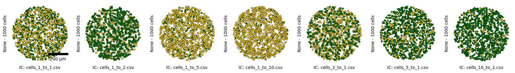
# Snapshots of the initial condition
fig, axes = plt.subplots(1,len(ICs), figsize=(21, 3), sharex=True, sharey=True)
ref_samples = df_mean_normalized_rmsd.index[df_mean_normalized_rmsd['Inactive_rule'].isna()].sort_values(ascending=True).tolist()
df_qois_data_selected = load_output(db_file, sample_ids=ref_samples, replicate_ids=[particular_replicate_id], load_data=True)
for i, IC in enumerate(ICs):
        mcds = df_qois_data_selected[df_qois_data_selected['SampleID'] == ref_samples[i]].iloc[particular_replicate_id]['Data'][0]
        df_cell = mcds.get_cell_df()
        plot_cells_2D(df_cell, color_dic, axes[i], scale_bar=True if (i==0) else False)
        # Set axis labels and ticks
        axes[i].set(xlabel=f'IC: {df_mean_normalized_rmsd.loc[ref_samples[i], "IC_file"]}', ylabel=f'{df_mean_normalized_rmsd.loc[ref_samples[i], "Inactive_rule"]} - {df_cell.shape[0]} cells')
        print(f"{ref_samples[i]} - IC: {df_mean_normalized_rmsd.loc[ref_samples[i], 'IC_file']}, Inactive rule: {df_mean_normalized_rmsd.loc[ref_samples[i], 'Inactive_rule']}, Cell count: {df_cell.shape[0]}")
plt.savefig('IC_Snapshots.svg', format='svg')

0 - IC: cells_1_to_1.csv, Inactive rule: None, Cell count: 1000
1 - IC: cells_1_to_2.csv, Inactive rule: None, Cell count: 1000
2 - IC: cells_1_to_5.csv, Inactive rule: None, Cell count: 1000
3 - IC: cells_1_to_10.csv, Inactive rule: None, Cell count: 1000
4 - IC: cells_2_to_1.csv, Inactive rule: None, Cell count: 1000
5 - IC: cells_5_to_1.csv, Inactive rule: None, Cell count: 1000
6 - IC: cells_10_to_1.csv, Inactive rule: None, Cell count: 1000

---

This notebook reproduces the rule inactivation analysis from Johnson et al. 2025. The ranked RMSD table identifies which behavioral rules most strongly influence the model outputs across different tumor-to-fibroblast seeding ratios.