Example 4: Global Sensitivity Analysis — Sobol with MPI
This notebook runs the same Sobol sensitivity analysis as ex3 but uses MPI (Message Passing Interface) for distributed execution across multiple compute nodes or cores. The simulation script is ex4_runSA_MPI.py — a plain Python file using the same ModelAnalysisContext API with parallel_method='inter-node'. The notebook launches it via %%bash and then loads results from the shared database.
Multi-task (ex3) vs MPI (ex4):
Multi-task (ex3) |
MPI (ex4) |
|
|---|---|---|
Launch |
Python API |
|
Scope |
Single machine |
Multiple nodes |
Setup |
No extra config |
Requires MPI installation |
Best for |
Laptops, workstations |
HPC clusters |
Model: asymmetric_division — stem cell division with reparameterized probabilities (prob. progenitor_2 = 1 − prob. progenitor_1).
Parameters explored:
cycle_duration_stem_cell— stem cell cycle durationasym_div_to_prog_1_sat— saturation probability of dividing into progenitor_1asym_div_to_prog_2_sat— saturation probability of dividing into progenitor_2
Run simulations via MPI
Each MPI rank picks up its share of the sample list and writes results to the shared database independently.
%%bash
mpiexec -n 8 python ex4_runSA_MPI.py
Initializing MPI job with 8 processes...
PhysiCell already exists at: PhysiCell-master
Skipping download. Use force_download=True to override.
Generated 48 samples using Sobol
Inserting parameter: cycle_duration_stem_cell with properties: {'lower_bound': 1152.0, 'upper_bound': 1728.0, 'ref_value': 1440.0, 'perturbation': None}
Inserting parameter: asym_div_to_prog_1_sat with properties: {'lower_bound': 0.0, 'upper_bound': 1.0, 'ref_value': 0.0, 'perturbation': None}
Inserting {'frac_proj1_cells': None, 'frac_proj2_cells': None, 'run_time_sec': None} QoIs into the database
Simulations completed and results stored in the database: ex4_PhysiCell_SA_MPI.db.
Load results and compute summary statistics
# Load results from the database
from uq_physicell.model_analysis import calculate_qoi_statistics
import warnings

warnings.filterwarnings('ignore')  # Suppress all warnings for cleaner output
# Load the results
db_path = "ex4_PhysiCell_SA_MPI.db"
qoi_funcs = {'frac_proj1_cells':None, 'frac_proj2_cells':None, 'run_time_sec':None}
df_qois_mean, df_qois_std, df_qois_mcse = calculate_qoi_statistics(db_path, qoi_funcs)
display(df_qois_mean)
No QoI data provided, calculating QoIs from the database...
All samples in Samples table have corresponding entries in Output table.
Extracting QoIs from DataFrame...
| frac_proj1_cells_0 | frac_proj2_cells_0 | run_time_sec_0 | time_0 | |
|---|---|---|---|---|
| SampleID | ||||
| 0 | 0.843984 | 0.125880 | 10.825394 | 2880.01 |
| 1 | 0.896023 | 0.073295 | 11.204853 | 2880.01 |
| 2 | 0.651961 | 0.317536 | 11.537088 | 2880.01 |
| 3 | 0.661141 | 0.309091 | 10.035426 | 2880.01 |
| 4 | 0.894974 | 0.074299 | 9.719086 | 2880.01 |
| 5 | 0.614583 | 0.354356 | 10.210138 | 2880.01 |
| 6 | 0.680871 | 0.288447 | 10.976077 | 2880.01 |
| 7 | 0.663192 | 0.306103 | 10.264580 | 2880.01 |
| 8 | 0.780370 | 0.190008 | 9.784336 | 2880.01 |
| 9 | 0.771402 | 0.197727 | 9.758274 | 2880.01 |
| 10 | 0.635649 | 0.333468 | 9.517483 | 2880.01 |
| 11 | 0.780147 | 0.189338 | 10.039442 | 2880.01 |
| 12 | 0.799209 | 0.170477 | 10.289918 | 2880.01 |
| 13 | 0.836292 | 0.134434 | 10.506709 | 2880.01 |
| 14 | 0.702639 | 0.267537 | 10.712825 | 2880.01 |
| 15 | 0.752590 | 0.217072 | 9.702209 | 2880.01 |
| 16 | 0.884388 | 0.085096 | 10.094876 | 2880.01 |
| 17 | 0.711582 | 0.258450 | 12.379703 | 2880.01 |
| 18 | 0.705426 | 0.264439 | 10.686780 | 2880.01 |
| 19 | 0.684894 | 0.285327 | 9.994548 | 2880.01 |
| 20 | 0.841756 | 0.127919 | 10.427948 | 2880.01 |
| 21 | 0.854501 | 0.115185 | 10.720837 | 2880.01 |
| 22 | 0.683389 | 0.286643 | 9.708683 | 2880.01 |
| 23 | 0.858560 | 0.110735 | 10.227116 | 2880.01 |
| 24 | 0.826203 | 0.143850 | 10.323526 | 2880.01 |
| 25 | 0.802217 | 0.168688 | 11.474282 | 2880.01 |
| 26 | 0.926637 | 0.042279 | 10.585155 | 2880.01 |
| 27 | 0.938957 | 0.030338 | 10.153952 | 2880.01 |
| 28 | 0.799566 | 0.170120 | 9.704243 | 2880.01 |
| 29 | 0.930822 | 0.037915 | 10.516060 | 2880.01 |
| 30 | 0.725824 | 0.243672 | 10.657874 | 2880.01 |
| 31 | 0.718596 | 0.250119 | 10.342664 | 2880.01 |
| 32 | 0.728855 | 0.241534 | 10.072137 | 2880.01 |
| 33 | 0.705235 | 0.264754 | 9.897537 | 2880.01 |
| 34 | 0.688000 | 0.281485 | 10.426809 | 2880.01 |
| 35 | 0.718530 | 0.250196 | 10.252921 | 2880.01 |
| 36 | 0.956617 | 0.012311 | 10.453640 | 2880.01 |
| 37 | 0.963972 | 0.006061 | 11.375506 | 2880.01 |
| 38 | 0.798702 | 0.170593 | 10.119175 | 2880.01 |
| 39 | 0.776225 | 0.193460 | 10.426868 | 2880.01 |
| 40 | 0.969508 | 0.000000 | 10.063891 | 2880.01 |
| 41 | 0.817536 | 0.151961 | 9.865496 | 2880.01 |
| 42 | 0.626549 | 0.342758 | 10.799564 | 2880.01 |
| 43 | 0.732264 | 0.237233 | 10.376397 | 2880.01 |
| 44 | 0.649075 | 0.320611 | 10.482474 | 2880.01 |
| 45 | 0.649115 | 0.320180 | 9.848048 | 2880.01 |
| 46 | 0.682955 | 0.286553 | 10.143365 | 2880.01 |
| 47 | 0.665809 | 0.303877 | 10.556484 | 2880.01 |
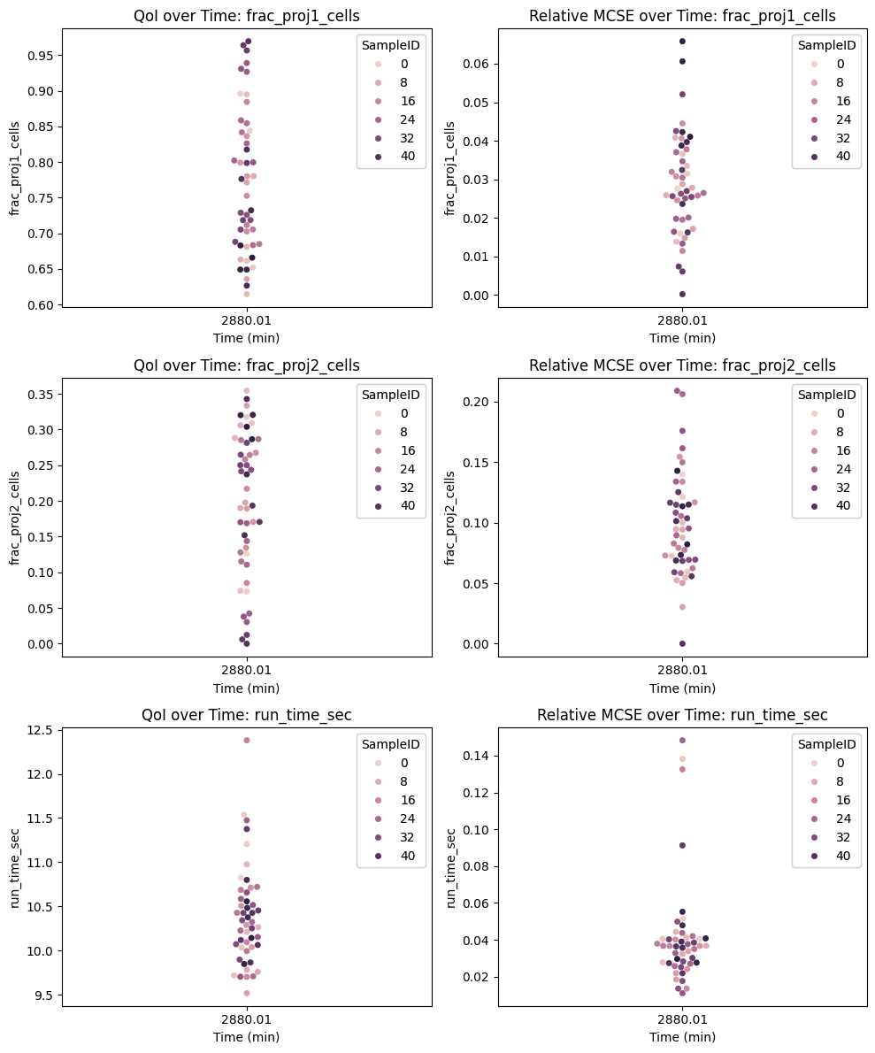
QoI over time and relative MCSE
import matplotlib.pyplot as plt
from uq_physicell.model_analysis import plot_qoi_over_time

fig, axes = plt.subplots(len(qoi_funcs.keys()), 2, figsize=(10, 4*len(qoi_funcs.keys())))
for ax_id, qoi_name in enumerate(qoi_funcs.keys()):
     # Plot QoI time series
    plot_qoi_over_time(df_qois_mean, qoi_name, axes[ax_id,0])
    axes[ax_id,0].set_title(f"QoI over Time: {qoi_name}")
    # Plot mcse
    plot_qoi_over_time(df_qois_mcse, qoi_name, axes[ax_id,1])
    axes[ax_id,1].set_title(f"Relative MCSE over Time: {qoi_name}")

# Ensure proper layout and save the figure
plt.tight_layout()  # This will automatically adjust spacing to prevent overlaps
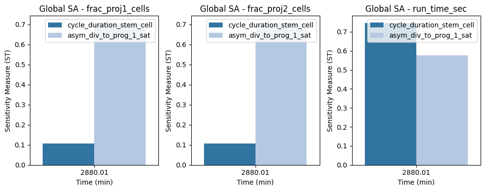
Sobol sensitivity indices (S1 and ST)
from uq_physicell.model_analysis import get_sa_results,load_parameter_space, plot_global_sa_results

sa_method = "Sobol Sensitivity Analysis"
qoi_names = list(qoi_funcs.keys())
sa_results, qoi_time_values = get_sa_results(db_path, qoi_names, df_qois_mean, sa_method)
param_names = load_parameter_space(db_path)['ParamName'].tolist()  # Load parameter names from the database

# Plot Global SA results
fig, axes = plt.subplots(1, 3, figsize=(10, 4))
for ax_id, qoi_name in enumerate(qoi_names):
    plot_global_sa_results(param_names, sa_method, qoi_time_values, sa_results, qoi_name, 'ST' , axes[ax_id])
    axes[ax_id].set_title(f'Global SA - {qoi_name}')
    axes[ax_id].legend(loc='best')

plt.tight_layout()
Warning: Could not convert perturbation (None) to float for parameter cycle_duration_stem_cell.
Warning: Could not convert perturbation (None) to float for parameter asym_div_to_prog_1_sat.
Running sensitivity analysis with method: Sobol Sensitivity Analysis
Running Sobol Sensitivity Analysis for QoI: frac_proj1_cells and time: 2880.01
Running Sobol Sensitivity Analysis for QoI: frac_proj2_cells and time: 2880.01
Running Sobol Sensitivity Analysis for QoI: run_time_sec and time: 2880.01
Next: ex5 demonstrates local sensitivity analysis using One-At-a-Time (OAT) sampling — a lighter approach for screening which parameters matter before running a full Sobol analysis.